1Overview
This appendix provides essential background on modal analysis for readers less familiar with structural dynamics. Modal analysis transforms coupled equations of motion into independent SDOF systems, enabling efficient solution of complex structural vibration problems. The concepts covered here support the frequency-domain analysis and system identification techniques presented in Chapters 3 and 4.
Understanding modal analysis is crucial for structural health monitoring because structural damage manifests as changes in natural frequencies, damping ratios, and mode shapes. By decomposing structural response into modal contributions, we can isolate and track individual modes over time to detect damage.
2Equations of Motion for MDOF Systems
2.1General Matrix Form
Consider a linear structural system with degrees of freedom subjected to time-varying forces. The equation of motion is:
where:
is the mass matrix
is the damping matrix
is the stiffness matrix
is the displacement response vector
is the applied force vector
2.2The Coupling Problem
Eq. (1) represents a system of second-order differential equations. Each row corresponds to one degree of freedom, but these equations cannot be solved independently because the response of other DOFs contributes to each equation. We say the equations are coupled. To illustrate coupling, consider a simple 2-DOF system:
The off-diagonal terms and couple the two equations. Solving requires knowing and vice versa.
3Modal Coordinate Transformation
3.1The Mode Shape Matrix
The key insight of modal analysis is that there exists a coordinate transformation that decouples the equations. We assume a special matrix called the mode shape matrix, where each column is an independent vector called a mode shape:
These mode shapes form an orthogonal basis for , meaning they satisfy:
3.2Modal Expansion
We express the physical displacement response as a linear combination of mode shapes weighted by time-varying modal coordinate responses:
where is the modal coordinate vector. This is called modal expansion because each DOF response is the sum of all modal coordinate responses scaled by the mode shape components.
3.3Deriving Decoupled Equations
Pre-multiply both sides by :
Due to the orthogonality of the mode shapes, , , and are diagonal matrices. This yields independent equations:
where the modal parameters are:
3.4Normalized Form
Dividing (8) by gives the standard form for each modal coordinate:
where:
is the natural frequency of mode (rad/s)
is the damping ratio of mode
Each modal equation is now an independent SDOF system. The solution for the response to an arbitrary modal force is given by Duhamel’s integral (convolution with the impulse response for that mode):
where is the SDOF unit impulse response function for mode :
and is the damped natural frequency of mode .
Thus, the physical response can be reconstructed from the modal contributions, each of which is solved using the above formula.
4Finding Mode Shapes: The Eigenvalue Problem
4.1Proportional Damping Assumption
To find the mode shape matrix that decouples the equations, we typically assume proportional damping (also called Rayleigh damping):
where and are constants. This assumption is reasonable for many structures and ensures that the same mode shapes diagonalize both and .
4.2Undamped Eigenvalue Problem
Under proportional damping, we can find mode shapes from the undamped problem:
Assuming harmonic motion leads to the generalized eigenvalue problem:
This yields:
eigenvalues , where are natural frequencies
eigenvectors , which are the mode shapes
4.3Python implementation
In Python, we solve this using NumPy’s scipy.linalg.eigh for generalized eigenvalue problems:
1 2 3 4 5 6 7 8 9 10 11 12import numpy as np from scipy import linalg # Solve generalized eigenvalue problem eigenvalues, eigenvectors = linalg.eigh(K, M) # Extract natural frequencies (rad/s) omega_n = np.sqrt(eigenvalues) f_n = omega_n / (2 * np.pi) # Convert to Hz # Mode shape matrix (columns are mode shapes) Phi = eigenvectors
The eigenvalues and eigenvectors are automatically sorted from lowest to highest frequency. The mode shapes have physical meaning—they describe the relative motion pattern of all DOFs when the structure vibrates at that mode’s natural frequency.
5Complete Modal Analysis Example
5.1Eigen Analysis
Consider a 4-DOF system representing a simplified multi-story building. The mass and stiffness matrices are:
import numpy as np
from scipy import linalg, signal
import pandas as pd
from IPython.display import display

# System parameters (4-story building model)
m = 1000  # kg per floor

# Mass matrix (diagonal)
M = m * np.eye(4)

# Stiffness matrix (N/m)
k = 1e6  # N/m
K = k * np.array([
    [ 2, -1,  0,  0],
    [-1,  2, -1,  0],
    [ 0, -1,  2, -1],
    [ 0,  0, -1,  1]
])

# Solve eigenvalue problem
eigenvalues, eigenvectors = linalg.eigh(K, M)

# Natural frequencies
omega_n = np.sqrt(eigenvalues)
f_n = omega_n / (2 * np.pi)

# Mode shape matrix (normalized)
Phi = eigenvectors

# Create results dataframe
results_df = pd.DataFrame({
    'Mode': [f'Mode {i+1}' for i in range(4)],
    'ω (rad/s)': [f'{w:.2f}' for w in omega_n],
    'f (Hz)': [f'{f:.3f}' for f in f_n],
    'Period (s)': [f'{1/f:.3f}' for f in f_n]
})

results_df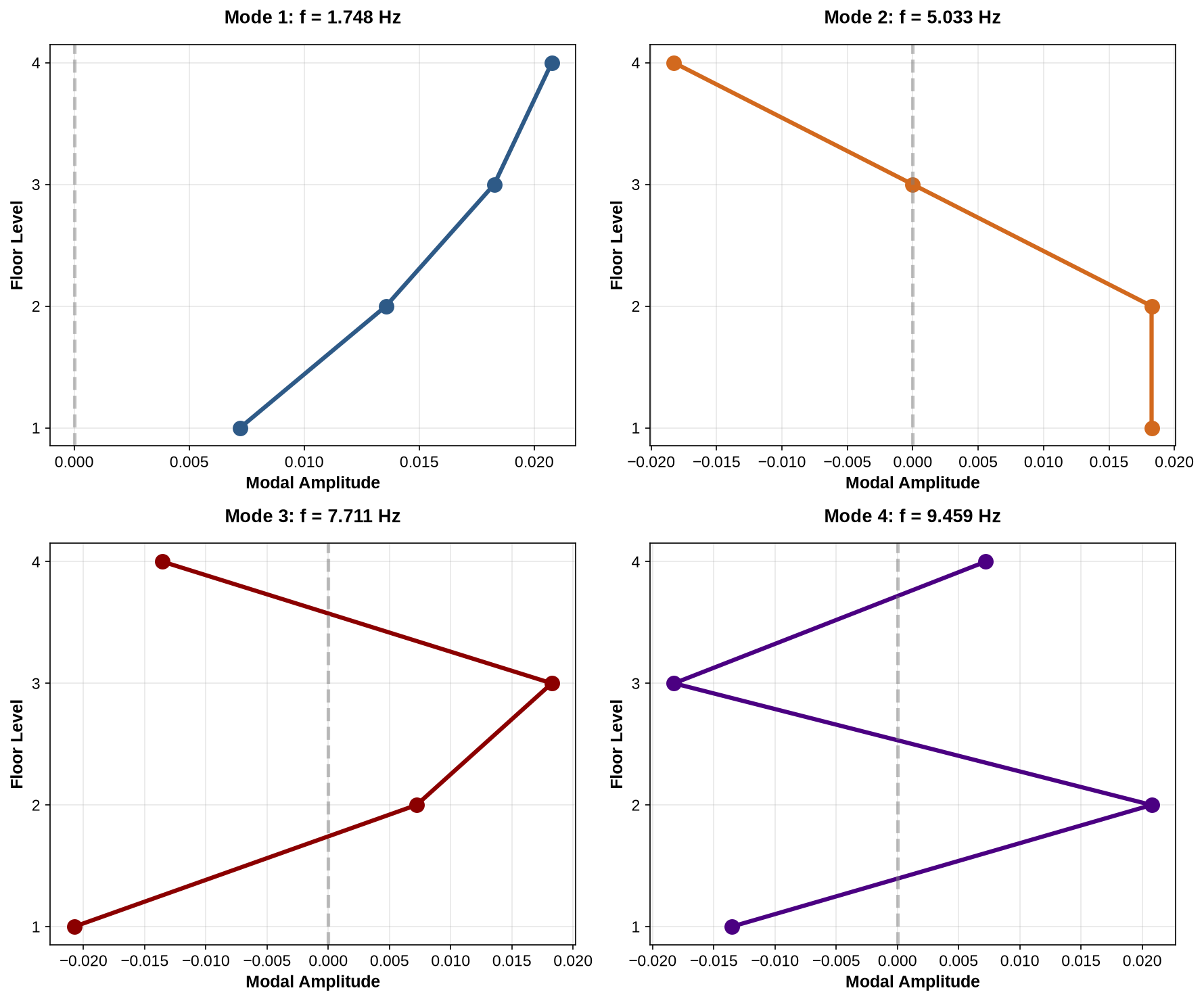
Figure 1:Mode shapes for 4-DOF system. Each mode represents a distinct vibration pattern with specific relative motions between DOFs.
Figure 1 shows the four mode shapes. Mode 1 (lowest frequency) shows all floors moving in the same direction—this is the fundamental sway mode. Mode 2 shows the upper floors moving opposite to lower floors. Higher modes show increasingly complex patterns with more zero-crossings (node points).
5.2Modal Decomposition and Response Solution
Now we’ll solve the system’s response to applied forces using modal superposition. The steps are:
Transform forces to modal coordinates:
Solve each modal equation independently using Duhamel’s integral
Reconstruct physical response:
# Time parameters
dt = 0.001  # s
t = np.arange(0, 5, dt)
N = len(t)

# Applied force (harmonic force on top floor)
u = np.zeros((4, N))
f_force = 1.2  # Hz (near Mode 1)
u[3, :] = 5000 * np.sin(2 * np.pi * f_force * t)  # N

# Modal damping ratios (assumed)
zeta = np.array([0.02, 0.025, 0.03, 0.035])

# Solve using modal superposition
q = np.zeros((4, N))  # Modal coordinates
x = np.zeros((4, N))  # Physical displacements

for r in range(4):
    # Modal parameters
    phi_r = Phi[:, r]
    omega_nr = omega_n[r]
    zeta_r = zeta[r]
    omega_dr = omega_nr * np.sqrt(1 - zeta_r**2)

    # Modal mass
    m_r = phi_r.T @ M @ phi_r

    # Modal force
    u_r = phi_r.T @ u

    # Duhamel's integral (convolution with impulse response)
    h_r = (1 / (m_r * omega_dr)) * np.exp(-zeta_r * omega_nr * t) * np.sin(omega_dr * t)

    # Convolve modal force with impulse response
    q[r, :] = signal.convolve(u_r, h_r, mode='same') * dt

# Reconstruct physical response
x = Phi @ q

print(f"\nMaximum displacement at top floor: {np.max(np.abs(x[3,:]))*1000:.2f} mm")
Maximum displacement at top floor: 48.75 mm
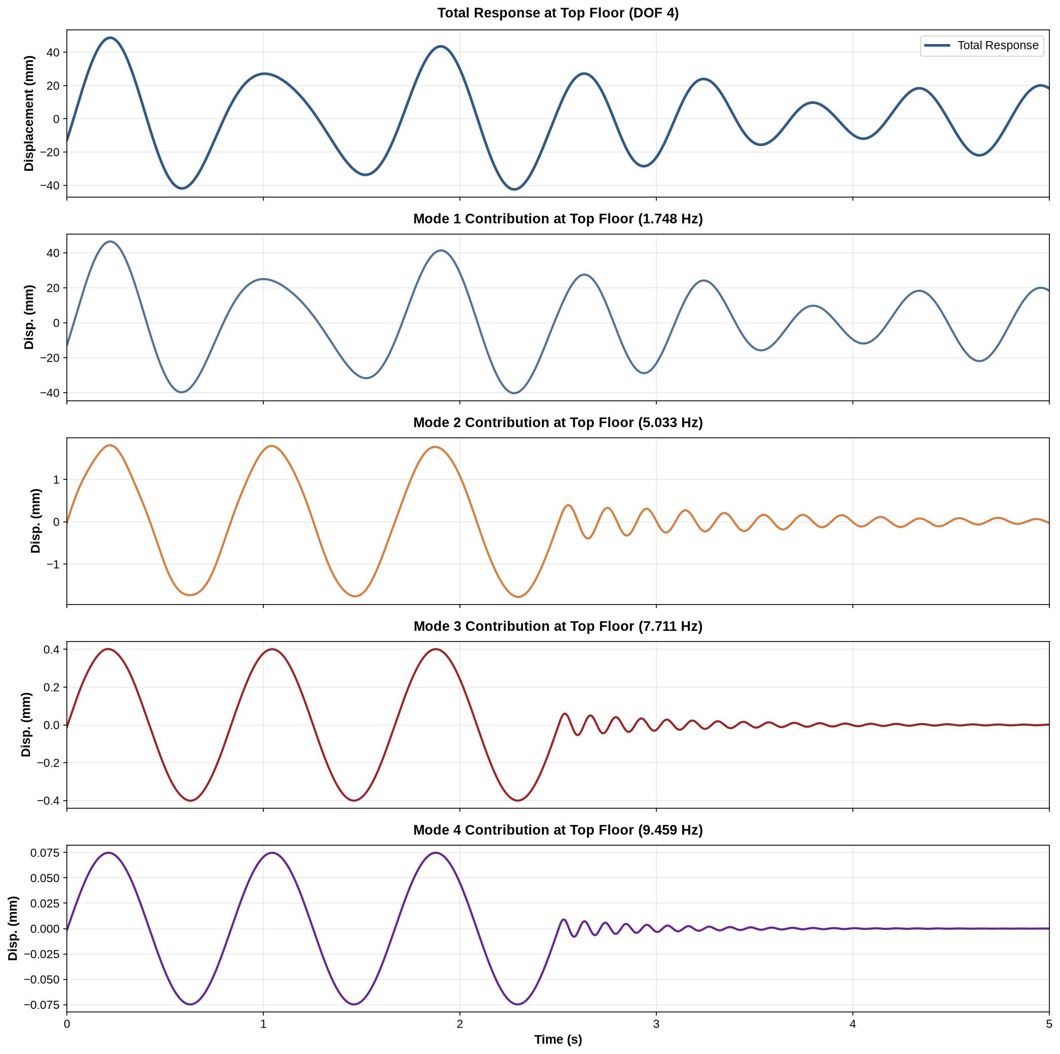
Figure 2:Physical response at top floor (DOF 4) showing the total response and the individual modal contributions.
6Physical Interpretation
6.1Why Modal Analysis Works
Modal analysis succeeds because structures have preferred vibration patterns (modes) determined by their mass and stiffness distribution. When excited, a structure responds as a combination of these patterns, each oscillating at its natural frequency with its own damping.
Think of mode shapes as the structure’s natural vocabulary for motion. Any arbitrary deformation can be expressed as a combination of mode shapes, just as any sound can be expressed as a combination of pure tones (Fourier series).
6.2Modal Participation
Not all modes contribute equally to every loading condition. The modal force determines how strongly mode is excited:
If aligns with the force distribution, is large (strong participation)
If is orthogonal to the force distribution, (weak participation)
In our example, the force was applied only at the top floor. Mode 1 has large amplitude at the top floor, so it was strongly excited. This is why the first mode dominated the response.
6.3Truncation and Model Reduction
For large systems, we often don’t need all modes. We can truncate the modal expansion to include only the first significant modes:
This model reduction dramatically decreases computational cost while maintaining accuracy for low-frequency response. For structural dynamics, typically because higher modes contribute negligibly to typical loading conditions.
6.4Damping Ratio Ranges
While mass and stiffness can be calculated from geometry and material properties, damping is difficult to predict theoretically. Damping ratios are typically:
0.5–2% for steel structures
2–5% for reinforced concrete
3–7% for timber structures
6.5Connection to Experimental Modal Analysis
The modal parameters (, , ) found from analytical models can be compared with experimental measurements from:
Frequency Domain Decomposition (FDD) - extracts mode shapes from vibration data
Peak Picking - identifies natural frequencies from power spectral densities
7Modal Analysis in Finite Element Software
7.1OpenSees and OpenSeesPy
OpenSees is a powerful, open-source finite element framework originally developed at UC Berkeley for earthquake engineering research. OpenSeesPy is the Python interface to OpenSees, providing full access to OpenSees capabilities through intuitive Python commands. This allows seamless integration with Python’s scientific ecosystem (NumPy, SciPy, Matplotlib) for pre-processing, analysis, and post-processing.
7.2Performing Eigenvalue Analysis in OpenSeesPy
Once a finite element model is built in OpenSeesPy (nodes, elements, boundary conditions, and mass assignment), performing modal analysis requires just a few lines of code:
1 2 3 4 5 6 7 8 9 10 11 12 13 14 15 16 17 18 19 20 21import openseespy.opensees as ops import numpy as np # Perform eigenvalue analysis (extract 5 modes) eigenvalues = ops.eigen(5) # Extract natural frequencies (rad/s) omega_n = np.sqrt(np.abs(eigenvalues)) f_n = omega_n / (2 * np.pi) # Convert to Hz # Extract mode shapes node_tags = ops.getNodeTags() # Get all node IDs mode_shapes = [] for mode_num in range(1, 6): # Modes 1 to 5 mode_shape = [] for node_tag in node_tags: # Get vertical displacement (DOF 2) for this mode disp = ops.nodeEigenvector(node_tag, mode_num, 2) mode_shape.append(disp) mode_shapes.append(mode_shape)
7.3Modal Analysis Utility for Bridge Structures
To simplify modal analysis for continuous beam structures (bridges), I have provided a utility class that automates the entire workflow—from model building to mode shape visualization. The utility is particularly useful for teaching and quick parametric studies.
Modal Analysis Utility Code (click to expand)
1 2 3 4 5 6 7 8 9 10 11 12 13 14 15 16 17 18 19 20 21 22 23 24 25 26 27 28 29 30 31 32 33 34 35 36 37 38 39 40 41 42 43 44 45 46 47 48 49 50 51 52 53 54 55 56 57 58 59 60 61 62 63 64 65 66 67 68 69 70 71 72 73 74 75 76 77 78 79 80 81 82 83 84 85 86 87 88 89 90 91 92 93 94 95 96 97 98 99 100 101 102 103 104 105 106 107 108 109 110 111 112 113 114 115 116 117 118 119 120 121 122 123 124 125 126 127 128 129 130 131 132 133 134 135 136 137 138 139 140 141 142 143 144 145 146 147 148 149 150 151 152 153 154 155 156 157 158 159 160 161 162 163 164 165 166 167 168 169 170 171 172 173 174 175 176 177 178 179 180 181 182 183 184 185 186 187 188 189 190 191 192 193 194 195 196 197 198 199 200 201 202 203 204 205 206 207 208 209 210 211 212 213 214 215 216 217 218 219 220 221 222 223 224 225 226 227 228 229 230 231 232 233 234 235 236 237 238 239 240 241 242 243 244 245 246 247 248 249 250 251 252 253 254 255 256 257 258 259 260 261 262 263 264 265 266 267 268 269 270 271 272 273 274 275 276 277 278 279 280 281 282 283 284 285 286 287 288 289 290 291 292 293 294 295 296 297 298 299 300 301 302 303 304 305""" Modal Analysis Utility - Simplified Version Clean teaching tool for eigenvalue analysis using OpenSeesPy. """ import numpy as np import matplotlib.pyplot as plt from scipy.interpolate import CubicSpline import openseespy.opensees as ops class ModalAnalysis: """Simple modal analysis for continuous beam structures.""" def __init__(self, spans, supports, E=25e9, rho=2500, A=8.0, I=2.67, mesh_size=0.5, I_factors=None): """ Initialize modal analysis. Parameters: - spans: List of span lengths [30, 50] - supports: Support types ['hinge', 'roller', 'roller'] - E: Elastic modulus (Pa) - rho: Density (kg/m³) - A: Cross-sectional area (m²) - I: Moment of inertia (m⁴) - mesh_size: Element length (m) - I_factors: Optional list of scaling factors for moment of inertia per span """ self.spans = spans self.supports = supports self.E = E self.rho = rho self.A = A self.I = I self.mesh_size = mesh_size if I_factors is not None: if len(I_factors) != len(spans): raise ValueError("I_factors must match the number of spans") self.I_factors = [float(val) for val in I_factors] else: self.I_factors = [1.0] * len(spans) if len(supports) != len(spans) + 1: raise ValueError(f"Need {len(spans) + 1} supports for {len(spans)} spans") self.total_length = sum(spans) self.support_positions = [0] + [sum(spans[:i+1]) for i in range(len(spans))] self.frequencies = None self.periods = None self.mode_shapes = None self.node_positions = None def analyze(self, n_modes=5, figsize=(14, 10), plot=True): """ Perform eigenvalue analysis and plot mode shapes. Parameters: - n_modes: Number of modes to extract - figsize: Figure size (width, height) - plot: Whether to generate plots of the mode shapes """ # Initialize OpenSees ops.wipe() ops.model('BasicBuilder', '-ndm', 2, '-ndf', 3) # Create nodes for each span (don't duplicate at span interfaces) current_node_tag = 1 span_node_tags = [] all_node_positions = [] for i, (span_start, span_end) in enumerate(zip(self.support_positions[:-1], self.support_positions[1:])): span_length = span_end - span_start n_seg = int(np.ceil(span_length / self.mesh_size)) dx = span_length / n_seg this_span_nodes = [] for j in range(n_seg + 1): xcoord = span_start + j * dx if i == 0 or j != 0: # Don't duplicate nodes at span interfaces ops.node(current_node_tag, xcoord, 0.0) all_node_positions.append(xcoord) this_span_nodes.append(current_node_tag) current_node_tag += 1 else: # Use last node from previous span this_span_nodes.append(span_node_tags[-1][-1]) span_node_tags.append(this_span_nodes) # Get all unique node tags and positions all_node_tags = [] final_positions = [] for span_nodes in span_node_tags: for node_tag in span_nodes: if node_tag not in all_node_tags: all_node_tags.append(node_tag) coord = ops.nodeCoord(node_tag) final_positions.append(coord[0]) # Sort by position sorted_indices = np.argsort(final_positions) all_node_tags = [all_node_tags[i] for i in sorted_indices] self.node_positions = np.array([final_positions[i] for i in sorted_indices]) # Apply boundary conditions for idx, support_x in enumerate(self.support_positions): node_idx = np.argmin(np.abs(self.node_positions - support_x)) support_node = all_node_tags[node_idx] support_type = self.supports[idx].lower() if support_type == 'hinge': ops.fix(support_node, 1, 1, 0) elif support_type == 'roller': ops.fix(support_node, 0, 1, 0) elif support_type == 'fixed': ops.fix(support_node, 1, 1, 1) # Create beam elements transf_tag = 1 ops.geomTransf('Linear', transf_tag) element_tag = 1 for span_idx, span_nodes in enumerate(span_node_tags): for j in range(len(span_nodes) - 1): nd_i = span_nodes[j] nd_j = span_nodes[j + 1] span_I = self.I * self.I_factors[span_idx] ops.element('elasticBeamColumn', element_tag, nd_i, nd_j, self.A, self.E, span_I, transf_tag) element_tag += 1 # Assign nodal mass (distributed from elements) linear_mass = self.rho * self.A for span_nodes in span_node_tags: for j in range(len(span_nodes) - 1): nd_i = span_nodes[j] nd_j = span_nodes[j + 1] xi = ops.nodeCoord(nd_i)[0] xj = ops.nodeCoord(nd_j)[0] le = xj - xi # Get current mass (in case node is shared) current_mass_i = ops.nodeMass(nd_i)[1] if len(ops.nodeMass(nd_i)) > 1 else 0.0 current_mass_j = ops.nodeMass(nd_j)[1] if len(ops.nodeMass(nd_j)) > 1 else 0.0 # Add half of element mass to each node ops.mass(nd_i, 0.0, current_mass_i + 0.5 * linear_mass * le, 0.0) ops.mass(nd_j, 0.0, current_mass_j + 0.5 * linear_mass * le, 0.0) # Perform eigenvalue analysis eigenvalues = ops.eigen(n_modes) # Extract modal properties omega = np.sqrt(np.abs(eigenvalues)) self.frequencies = omega / (2 * np.pi) self.periods = 1 / self.frequencies # Extract mode shapes at sorted node positions n_nodes = len(all_node_tags) self.mode_shapes = np.zeros((n_nodes, n_modes)) for mode in range(n_modes): for i, node_tag in enumerate(all_node_tags): disp = ops.nodeEigenvector(node_tag, mode + 1, 2) self.mode_shapes[i, mode] = disp # Normalize mode shapes for mode in range(n_modes): max_val = np.max(np.abs(self.mode_shapes[:, mode])) if max_val > 0: self.mode_shapes[:, mode] /= max_val result = { 'frequencies': self.frequencies.copy(), 'periods': self.periods.copy(), 'mode_shapes': self.mode_shapes.copy(), 'node_positions': self.node_positions.copy() } # Plot mode shapes if requested if plot: self._plot_mode_shapes(n_modes, figsize) return result def _plot_mode_shapes(self, n_modes, figsize): """Internal method to plot mode shapes.""" # Layout: 3x1 for 3 or fewer modes, nx2 for more than 3 if n_modes <= 3: n_rows = n_modes n_cols = 1 else: n_cols = 2 n_rows = int(np.ceil(n_modes / n_cols)) fig, axes = plt.subplots(n_rows, n_cols, figsize=figsize) # Handle axes array shape if n_modes == 1: axes = np.array([[axes]]) elif n_rows == 1: axes = axes.reshape(1, -1) elif n_cols == 1: axes = axes.reshape(-1, 1) for mode_idx in range(n_modes): row = mode_idx // n_cols col = mode_idx % n_cols ax = axes[row, col] mode_num = mode_idx + 1 mode_shape = self.mode_shapes[:, mode_idx] # Enforce zero at supports plot_x = self.node_positions.copy() plot_y = mode_shape.copy() for support_x in self.support_positions: support_idx = np.argmin(np.abs(self.node_positions - support_x)) plot_y[support_idx] = 0.0 # Smooth curve with spline unique_x, unique_indices = np.unique(plot_x, return_index=True) unique_y = plot_y[unique_indices] if len(unique_x) > 3: spline = CubicSpline(unique_x, unique_y) x_smooth = np.linspace(unique_x.min(), unique_x.max(), 500) y_smooth = spline(x_smooth) ax.plot(x_smooth, y_smooth, 'b-', linewidth=2, label='Mode Shape') else: ax.plot(unique_x, unique_y, 'b-', linewidth=2, label='Mode Shape') # Add support triangles for support_x in self.support_positions: triangle_height = 0.2 triangle = plt.Polygon([ [support_x - 1.5, -triangle_height], [support_x + 1.5, -triangle_height], [support_x, 0] ], color='green', alpha=0.6, zorder=5) ax.add_patch(triangle) # Add frequency and period text freq = self.frequencies[mode_idx] period = self.periods[mode_idx] ax.text(0.02, 0.98, f'f = {freq:.3f} Hz\nT = {period:.3f} s', transform=ax.transAxes, fontsize=10, verticalalignment='top', bbox=dict(boxstyle='round', facecolor='wheat', alpha=0.5)) # Formatting ax.set_xlim(-2, self.total_length + 2) ax.set_ylim(-1.05, 1.05) ax.axhline(y=0, color='k', linestyle='--', linewidth=0.5, alpha=0.3) ax.set_xlabel('Position (m)', fontsize=11) ax.set_ylabel('Amplitude', fontsize=11) ax.set_title(f'Mode {mode_num}', fontsize=12, fontweight='bold') ax.grid(True, alpha=0.3) # Hide unused subplots for idx in range(n_modes, n_rows * n_cols): row = idx // n_cols col = idx % n_cols axes[row, col].axis('off') plt.tight_layout() plt.show() def get_mode_shape_at_positions(self, positions, mode_num=1): """ Get mode shape values at specific positions using interpolation. Parameters: - positions: Array of positions along the beam - mode_num: Mode number (1-indexed) Returns: - Mode shape values at specified positions """ if self.mode_shapes is None: raise ValueError("No analysis results. Run analyze() first.") mode_idx = mode_num - 1 if mode_idx >= self.mode_shapes.shape[1]: raise ValueError(f"Mode {mode_num} not available") mode_shape = self.mode_shapes[:, mode_idx] # Enforce zero at supports for support_x in self.support_positions: support_idx = np.argmin(np.abs(self.node_positions - support_x)) mode_shape[support_idx] = 0.0 # Interpolate unique_x, unique_indices = np.unique(self.node_positions, return_index=True) unique_y = mode_shape[unique_indices] spline = CubicSpline(unique_x, unique_y) return spline(positions)
Requirements (click to expand)
# Modal Analysis Utility - Requirements
# ======================================
# Tested with Python 3.8 (Required for OpenSeesPy on Windows)

numpy==1.24.4
scipy==1.10.1
matplotlib==3.7.5
openseespy==3.3.0.1.1
openseespywin==3.3.0.1

# Installation Instructions:
# --------------------------
# 1. Ensure you have Python 3.8 installed
# 2. Create a virtual environment (recommended):
#    python -m venv .venv
# 3. Activate the virtual environment:
#    Windows: .venv\Scripts\activate
#    Linux/Mac: source .venv/bin/activate
# 4. Install requirements:
#    pip install -r requirements.txt
#
# Note: OpenSeesPy requires Python 3.8 on Windows
7.4Example: Two-Span Bridge Modal Analysis
The following example demonstrates how to use the modal analysis utility to extract natural frequencies and mode shapes for a two-span continuous bridge with a hinge support at the first support and roller supports at the second and third supports:
1 2 3 4 5 6 7 8 9 10 11 12 13 14 15 16 17 18 19 20import numpy as np from modal_analysis_utility import ModalAnalysis # Define structure spans = [30, 50] # Two spans: 30m and 50m supports = ['hinge', 'roller', 'roller'] # Support types # Material and section properties E = 25e9 # Elastic modulus (Pa) rho = 2500 # Density (kg/m³) A = 8.0 # Cross-sectional area (m²) I = 2.67 # Moment of inertia (m⁴) # Create analyzer and perform modal analysis modal = ModalAnalysis(spans, supports, E=E, rho=rho, A=A, I=I) modal.analyze(n_modes=4, save_filename='two_span_bridge_modes.png') # Access results print(f"Natural frequencies: {modal.frequencies} Hz") print(f"Periods: {modal.periods} s")
When you run this code, the utility automatically:
Builds the finite element model with proper meshing
Applies boundary conditions based on support types
Assigns distributed mass to nodes
Solves the eigenvalue problem
Normalizes mode shapes
Generates professional plots with frequency and period annotations
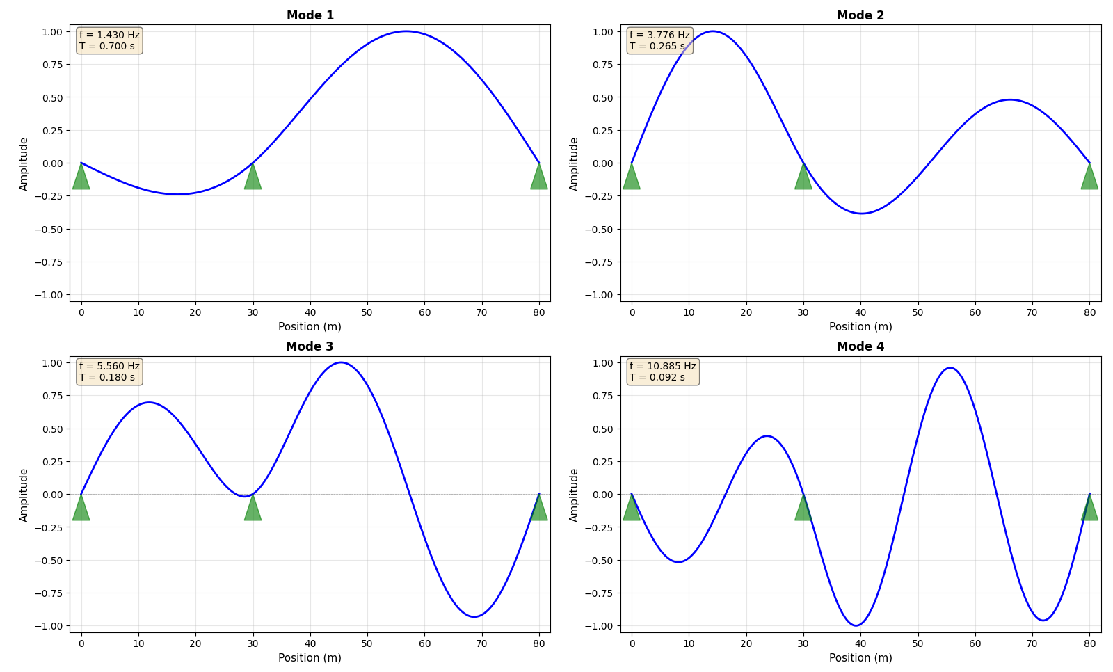
Figure 3:Modal analysis results for a two-span bridge (30m + 50m) showing the first four modes.
8Summary
Modal analysis transforms coupled MDOF equations into independent SDOF systems through:
Modal coordinate transformation:
Decoupling via orthogonality: Pre-multiplying by yields diagonal modal equations
Independent solution: Each modal equation is solved as an SDOF system
Reconstruction: Physical response is reconstructed via modal expansion
This approach enables efficient dynamic analysis of large structures and provides the theoretical foundation for frequency-domain system identification methods used in structural health monitoring. The natural frequencies, damping ratios, and mode shapes extracted through modal analysis serve as damage-sensitive features that change when structural properties degrade.