1Overview
Many sensor types are employed in SHM of bridges, each targeting different physical parameters and damage indicators. Global monitoring techniques use sensors (e.g. accelerometers) to capture overall structural behavior (such as modal frequencies and mode shapes), which are sensitive to stiffness changes in the bridge. Local monitoring techniques, in contrast, deploy sensors at specific critical locations (e.g. strain gauges or acoustic emission sensors) to detect localized phenomena like crack initiation, strain hotspots, or tendon failures. In practice, an SHM system may integrate hundreds of sensors to achieve full-scale monitoring of strain, displacement, temperature, acceleration, etc., on a large span bridge. The choice of sensor types and their placement is a critical design decision: it determines what structural performance attributes can be measured and which damage detection algorithms are applicable. In fact, accelerometers and strain gauges are among the most frequently used sensors in bridge SHM. Accelerometers are popular for their low cost and ease of use in measuring vibrations, while strain gauges directly capture deformation at critical points; other sensor types (e.g. acoustic emission, fiber-optic sensors, etc.) are typically used in more specialized roles to complement these primary sensors. Temperature sensors are also commonly included to help compensate for environmental influences on structural response. Overall, combining multiple sensing technologies provides a complete view of bridge health, from global stiffness down to local damage.
In the following sections, we explore the key sensor technologies used for bridge SHM, from traditional contact-based sensors to emerging smartphone-based sensing platforms. We will be focusing on their principles, advantages, limitations, and data acquisition (DAQ) considerations in civil engineering applications.
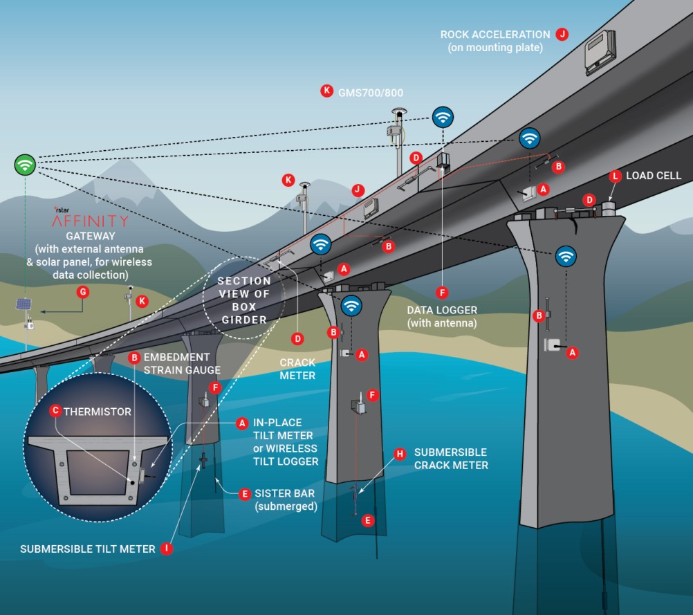
Figure 1:Bridge SHM sensor map showing typical placements [Source].
2The Evolution of Sensing in Bridge Monitoring
2.1Historical Context and Technological Development
The journey of structural sensing has been shaped by advances in materials science, electronics, and a deeper understanding of structural behavior.
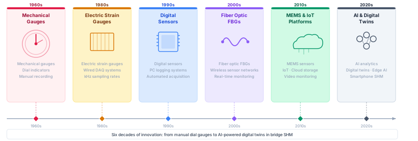
Figure 2:Timeline showing the evolution of sensor technologies in bridge monitoring from mechanical gauges to modern IoT-enabled systems.
The evolution shown in Figure 2 reveals several key technological transitions that have fundamentally changed how we approach structural monitoring. The earliest monitoring systems relied on mechanical gauges that required manual reading and provided only periodic snapshots of structural behavior. These systems, while rudimentary, established the foundation for understanding the importance of quantitative structural assessment.
The introduction of electrical strain gauges in the 1980s marked the first major shift in structural sensing. These sensors enabled continuous monitoring and remote data collection, though they were limited by analog signal processing and the need for extensive cabling infrastructure. The transition to digital sensors in the 2000s brought higher accuracy and the ability to integrate multiple sensor types into a single monitoring network.
The most recent developments have focused on wireless communication and smart sensor technologies that incorporate local processing capabilities. Today’s IoT-enabled sensors can perform edge computing, self-diagnosis, and adaptive sampling, representing a fundamental shift from passive sensing devices to intelligent monitoring nodes.
2.2Modern Sensing Requirements and Challenges
Contemporary bridge monitoring systems must address a complex set of requirements that extend far beyond simple data collection. Understanding these requirements is crucial for selecting appropriate sensor technologies and designing effective monitoring systems.
Long-term Reliability and Stability: Bridge monitoring systems are typically designed for operational lifespans of 20 to 50 years, during which sensors must maintain their calibration and continue providing accurate data. This requirement places significant constraints on sensor design, materials selection, and installation methods. Sensor drift, which refers to the gradual change in sensor output over time even when the measured parameter remains constant, becomes a critical consideration for long-term deployments.
Environmental Resilience: Bridge sensors must operate reliably in some of the harshest environmental conditions in engineering. Temperature cycling from -40°C to +50°C, humidity levels approaching 100%, exposure to de-icing salts, UV radiation, and mechanical vibration all contribute to an operating environment that can degrade sensor performance and shorten operational life. The selection of sensor technologies must carefully consider these environmental factors.
Multi-Parameter Monitoring Capability: Modern structural health monitoring requires simultaneous measurement of multiple parameters including strain, acceleration, displacement, temperature, humidity, wind speed, and in some cases, corrosion potential. The ability to integrate diverse sensor types into a coherent monitoring system while maintaining synchronization and data quality across all channels is essential for reliable structural assessment.
Real-time Data Processing and Communication: Contemporary monitoring systems must provide near real-time assessment of structural condition to enable rapid response to potentially dangerous situations. This requirement drives the need for high-speed data acquisition, reliable communication systems, and intelligent data processing algorithms that can distinguish between normal operational variations and genuine indicators of structural distress.
Cost-Effectiveness and Scalability: With thousands of bridges requiring monitoring in most developed countries, the cost per monitoring point becomes a critical factor in system design. Sensor technologies must provide an optimal balance between performance and cost, while also offering the scalability needed for network-wide deployment.
3Strain Gauges
Strain gauges are one of the most established sensor types in SHM, valued for their ability to directly measure strain (deformation) in structural elements. Bridges often develop critical strains under loads; by affixing strain gauges to high-stress regions (such as near supports, mid-span on girders, or around known hotspots), engineers can monitor actual strain levels and compare them to design limits or analytical predictions. This helps detect excessive load effects, distribution changes, or progressive deterioration (e.g. growing cracks or section loss) before failure occurs.
3.1Principle of Operation
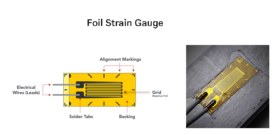
Most commonly, strain gauges are thin foil resistive sensors bonded to the surface of a structural member. As the member elongates or contracts under load, the strain gauge deforms with it, causing a change in the gauge’s electrical resistance proportional to the strain. This is quantified by the gauge factor (GF), defined as the ratio of fractional resistance change to strain:
where is the nominal resistance, its change, and the strain. For common metal foils, , so yields a fractional resistance change of . That is still a millivolt-level effect once embedded in a measurement circuit, which is why careful signal conditioning is essential. Figure 3 illustrates a strain gauge conceptually: a zig-zag pattern of conductive foil is bonded to the structure, so that even a tiny elongation stretches the foil and increases its electrical resistance. By wiring the gauge into a circuit, this resistance change can be measured and correlated to strain.
3.2Converting resistance to voltage: the Wheatstone bridge
Because is tiny, gauges are read in a Wheatstone bridge with a stable excitation and a differential measurement. The Wheatstone bridge is formed by two resistor dividers compared at their mid-nodes. If we label the arms as in Figure 4 (left leg top, bottom; right leg top, bottom) and excite with , the node voltages are:
The differential output is their difference,
Two immediate consequences follow:
Balance condition. when . Small fractional changes around that balance are what we measure as strain.
Ratiometric readout. Because the output scales with , report (in mV/V). This cancels most supply drift and lets different sites be compared directly.
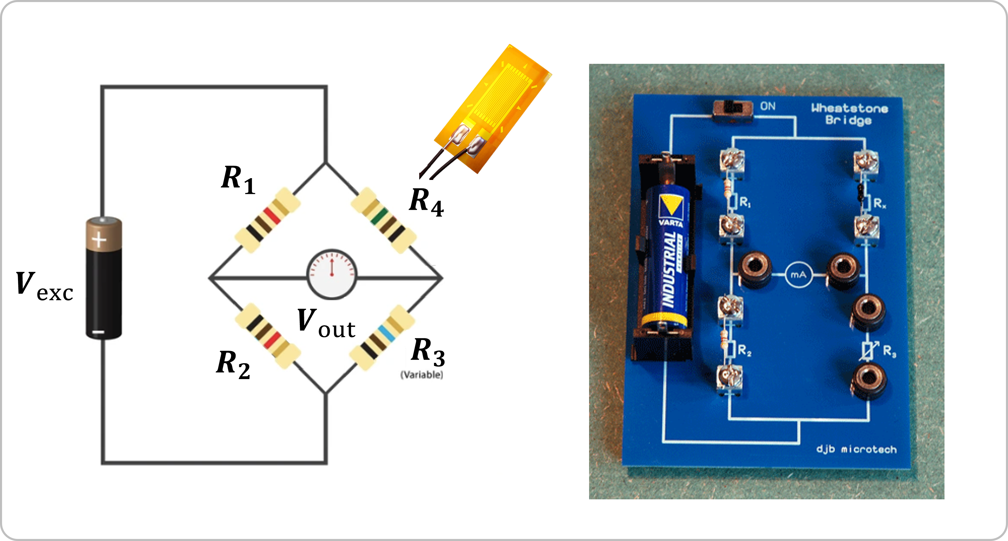
Figure 4:Wheatstone bridge.
Write each arm as where is the fractional change from strain and temperature. Linearizing (3) about balance gives
with . Wiring decides the signs, so you add the strain you want and cancel what you do not (temperature, axial leakage, bending leakage).
3.3Bridge configurations
Figure 5 gathers the six canonical Wheatstone-bridge configurations (configurations a–f) used with bonded foil strain gauges in SHM. In configuration (a) (quarter-bridge), a single active gauge occupies one arm (say ), the others are references, and the output reduces to the textbook small-signal result . This configuration is simple and useful for spot checks, but it offers no intrinsic temperature cancellation, so dummy gauges or explicit temperature channels are often required outdoors. Configuration (b) (“double-quarter” or diagonal) places two active gauges on opposite legs that experience the same axial strain; substituting and into (4) gives . Because bending typically produces equal-and-opposite strains at the two locations, its contribution largely cancels in this wiring, which is why diagonal bridges are preferred when axial strain is the target in the presence of flexure.
Configuration (c) is the bending half-bridge. Two gauges are mounted on opposite faces of a beam, one in tension and one in compression, and wired into adjacent arms so their mechanical signs add in the bridge. With and (other arms referenced), (4) yields for symmetric bending. Axial strain, having the same sign on both faces, cancels by construction; temperature terms are also strongly suppressed because the two active arms see nearly the same . Configuration (d) is the Poisson half-bridge, used when only one surface is accessible or when additional axial sensitivity and thermal rejection are needed. One gauge is longitudinal and the other transverse, placed in adjacent arms so that ; under the response becomes . The transverse element both boosts output and cancels much of the thermal drift because the gauges share the same leg.
The two full-bridge layouts extend these ideas to four actives. In configuration (e) (axial full-bridge), gauges are arranged so axial components add while bending cancels. Many practical patterns implement this as two Poisson half-bridges in opposite legs; the resulting gain is on the order of (often when both Poisson pairs contribute), with excellent temperature rejection. Configuration (f) (bending full-bridge) distributes two gauges in tension and two in compression such that their mechanical signs and the algebraic signs in (4) both produce addition; inserting , , , gives . This is the high-gain, high-immunity option when pure flexure is the quantity of interest: axial content cancels by symmetry, and thermal effects are minimized because all four arms are active and balanced.
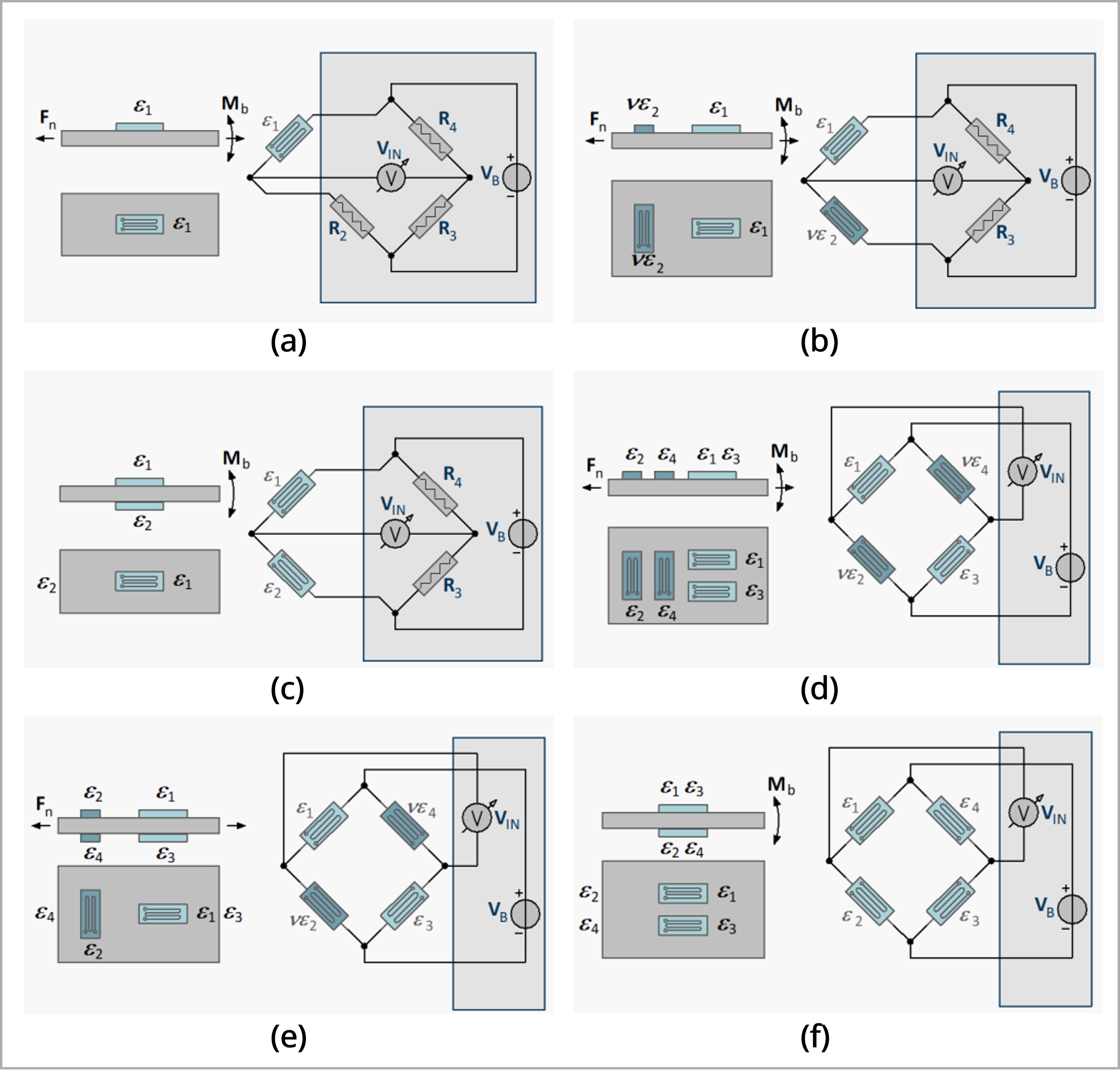
Figure 5:Six canonical Wheatstone-bridge layouts for strain gauges (a–f): quarter, diagonal (double-quarter), bending half-bridge, Poisson half-bridge, axial full-bridge, and bending full-bridge [Source].
3.4Multi-axis measurements with rosettes
A single foil gauge measures strain along one line. Often we need the two in-plane normal strains and the in-plane shear at the same point. A strain-gauge rosette does exactly that by placing three grids at known angles. The general geometry is shown in Figure 6.
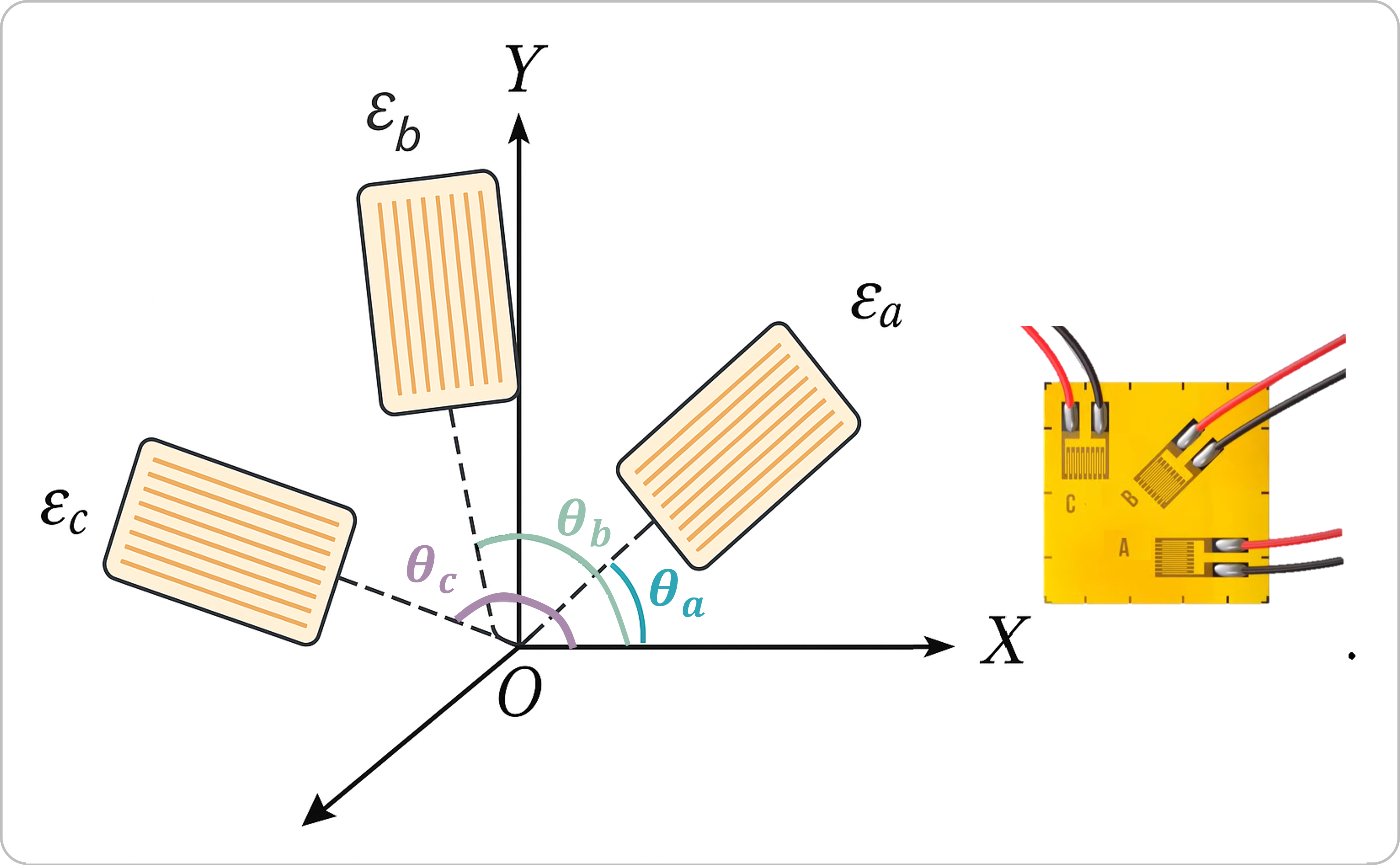
Figure 6:Strain rosette configuration for planar strain measurement.
Let be the in-plane strains in the global - axes. The strain along a direction making angle to the -axis is
If the rosette grids are at angles , the three measured strains satisfy a linear system
This formulation automatically handles any rosette rotation: just use the actual angles of the three grids in the global frame.
3.4.1Two common layouts
Rectangular rosette (grid at , at , at )
Delta rosette with the middle grid aligned to (i.e., ; this is the common “30–90–150°” placement in practice)
3.5Other types of strain gauges
Strain gauges come in various forms. Foil strain gauges (typically constantan or similar alloy) are inexpensive and widely used; they offer high strain sensitivity (microstrain-level resolution) but require careful installation (surface preparation and adhesive bonding) and protection from moisture. Vibrating wire strain gauges are another common type, especially for long-term monitoring in harsh environments. These consist of a tensioned wire embedded in the structure or attached to it; strain in the structure changes the tension in the wire, which in turn shifts its natural vibration frequency. By plucking the wire (electromagnetically) and measuring the frequency, strain can be inferred. Vibrating wire gauges are extremely stable over time and can operate in concrete or underwater, making them ideal for bridges, dams, and tunnels where electronic gauges might drift. Other strain-sensing technologies include fiber-optic strain gauges (covered in a later section) and newer materials like piezoresistive or MEMS gauges, but the foil and vibrating wire types remain the workhorses of bridge SHM. Each offers a means to directly measure how much a structural element is stretching or compressing under load, which is fundamental information for assessing structural health.
3.6Capabilities and practical limits
Strain gauges provide direct, quantitative measurements of strain, which is directly related to stress, a critical parameter for evaluating structural safety. They are highly sensitive; electrical foil gauges can detect strains on the order of ~1 or less (with proper instrumentation), allowing detection of minute structural changes. The technology is well-established and relatively low-cost; foil gauges and installation kits are readily available, and many civil structures have been instrumented with them for decades. Strain gauges have fast response and can capture both static and dynamic strain (up to high frequencies), making them suitable for monitoring live loads or vibrations. Vibrating wire gauges, in particular, excel in long-term stability: they can operate for many years with minimal drift, even in harsh conditions. Overall, strain gauges are versatile: they can be bonded to steel or concrete surfaces, embedded inside concrete (certain types), or attached to rebar, bolts, or other components. They effectively turn the structure into a sensor by measuring its deformation.
A key limitation is that strain gauges measure local strain at the sensor location only. They have a very small gage length (often ~5–10 mm for foil gauges), so they do not directly capture global deformations or conditions away from the installation point. Thus, many gauges may be needed to cover a large bridge, and interpreting what a single gauge’s reading means for overall structural health can be complex. Installation of bonded gauges requires surface preparation (smoothing, cleaning) and skillful bonding; errors in installation (poor adhesion, misalignment) can lead to bad data. They also require wiring for power and signal readout, which on large bridges means lengthy cables that can be susceptible to damage or signal noise. Temperature sensitivity is another issue: foil gauges are sensitive to thermal expansion of the substrate and their own gauge material, causing apparent strain changes with temperature. Techniques like using dummy temperature-compensation gauges or active temperature correction must be applied to distinguish load-induced strain from thermal effects. Moreover, in the long term, foil gauges can suffer drift due to creep in the adhesive or foil, and they must be protected against moisture and corrosion (often by coating with weather-proofing materials). Vibrating wire gauges avoid some issues of foil gauges (they handle temperature effects better and have long-term stability), but they are more expensive and require excitation and frequency measurement equipment. In summary, strain gauges provide crucial local data but come with practical challenges in installation, maintenance, and interpretation.
3.7Typical Specs & Performance
Foil strain gauges usually have nominal resistances of 120 Ω or 350 Ω and gauge factors around 2.0. They can reliably measure strain ranges of several thousand microstrain (enough to cover elastic strains in steel or concrete under normal loads) with resolution as fine as ~1 when using high-quality data acquisition. Some specialized gauges (e.g. semiconductor strain gauges) have much higher gauge factors (50–200) for greater sensitivity, but these are less common in civil structures due to stability issues. Vibrating wire gauges can measure strains in the same range (on the order of 1000s of ) and are known for long-term stability within a few microstrain over many years. Response frequency for foil gauges can be high (they can track dynamic strains up to kHz if properly instrumented), limited mainly by the adhesive and substrate dynamics. Vibrating wire gauges typically measure quasi-static strain (they may take a reading every few seconds) and are less suited to very fast-changing strain. Table 1 summarizes some key points.
Table 1:Strain Gauge Sensors: Key Features (typical values for civil SHM applications)
| Feature | Foil Strain Gauge | Vibrating Wire Gauge |
|---|---|---|
| Gauge Length | 5–10 mm (surface-mounted) | 150–250 mm (wire length within gauge) |
| Strain Range | ~±5000 (0.5% strain) | ~±3000 (depending on wire tension range) |
| Resolution | ~1 with 24-bit DAQ | ~1–5 (high stability over time) |
| Gauge Factor (Sensitivity) | ~2.0 (metal foil) | N/A (frequency output, not GF-based) |
| Temperature Effect | Significant (needs comp.) | Moderate (thermistor often included) |
| Installation | Bonded with epoxy; wired out | Embedded or surface-mounted; wired to datalogger |
| Notable Advantages | Low cost; fast response; widely used | Long-term stability; works in harsh environments |
| Notable Disadvantages | Localized measurement; prone to drift if not installed well; requires wiring and temp compensation | Slower sampling; more expensive; requires excitation and frequency readout |
4Accelerometers
Accelerometers are fundamental tools for global monitoring of bridge dynamics. They measure structural vibrations (accelerations) caused by traffic, wind, earthquakes, or other dynamic loads. These vibration signatures carry information about the bridge’s dynamic characteristics: for instance, the natural frequencies, mode shapes, and modal damping ratios of the structure can be extracted from acceleration data. Changes in these dynamic properties over time can indicate stiffness loss due to damage. Accelerometers are also used for real-time response monitoring: in extreme events like earthquakes or blast loads, peak accelerations and the ensuing vibrations provide crucial data on structural performance. Because they capture global behavior, accelerometers are typically deployed on a few strategic locations (e.g. mid-span and quarter-span on girders, tops of piers, etc.) to sense the dominant modes of vibration. Bridges often have low-frequency vibrations (fundamental modes in the range of ~0.5–10 Hz for large spans). Accelerometers tuned for these low frequencies can monitor the overall structural health. They are among the most widely used sensors in SHM because of their broad applicability and relatively simple installation.
4.1Principle of Operation
An accelerometer produces an electrical signal proportional to the acceleration of its base (the point where it’s attached to the structure). There are various types of accelerometers, but two are most relevant in civil SHM: piezoelectric accelerometers and MEMS accelerometers. A piezoelectric accelerometer contains a small mass attached to a piezoelectric crystal. When the device experiences acceleration, the mass exerts a force on the crystal (per Newton’s second law ), causing the crystal to deform and generate an electric charge or voltage. This output is proportional to the acceleration. Piezoelectric accelerometers are analog sensors known for their high frequency range and good sensitivity, but they generally cannot measure down to 0 Hz (static acceleration) because the charge dissipates; they are best for dynamic measurements. MEMS (Micro-Electro-Mechanical Systems) accelerometers, on the other hand, are tiny capacitive sensors where acceleration causes a microscopic proof mass to deflect, changing the capacitance of a circuit. This change can be converted to a voltage or digital reading. MEMS accelerometers (like those in smartphones and wireless sensor nodes) can measure static or DC accelerations (e.g. gravity or tilt) as well as dynamics, though often with higher noise at low frequencies.
No matter the type, the accelerometer essentially implements Newton’s second law. If is the internal mass and is its displacement relative to the casing, a basic model is: , where is the acceleration of the base. In a piezoelectric accelerometer, the piezo element provides the spring () and damping () and outputs a charge proportional to its deformation. The sensor is usually designed with a high natural frequency so that for the frequency range of interest, it behaves as a mass acting directly on a stiffness (i.e. output ). Accelerometers are often characterized by their sensitivity (e.g. 100 mV/g, meaning a acceleration produces output) and frequency response (range of frequencies over which they measure accurately). Figure 7 illustrates the typical accelerometers’ working principle. In essence, it’s a small box with an internal mass-spring system that converts motion into an electrical signal.
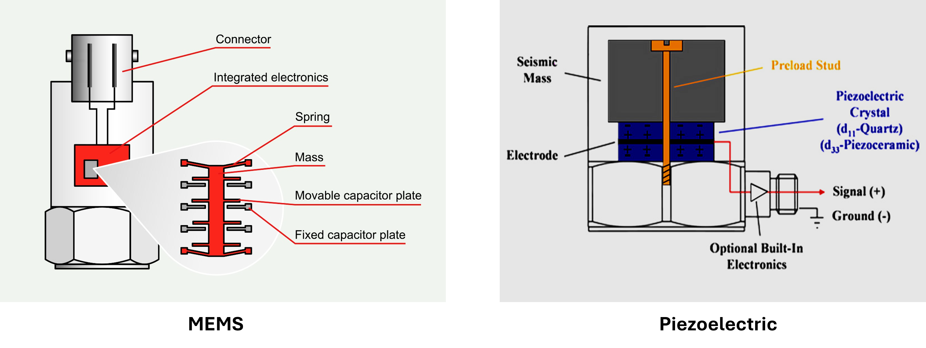
Figure 7:Conceptual diagrams of MEMS and Piezoelectric accelerometers. The device contains a proof mass on a spring (or piezoelectric element). When the bridge vibrates, the mass tends to stay behind, compressing the spring. The resulting deformation or charge output is proportional to the acceleration.
4.2Advantages and Disadvantages
Accelerometers are highly sensitive to a wide range of dynamic events. Good piezoelectric accelerometers can detect accelerations down to milli- or lower, sufficient to sense subtle ambient vibrations. They cover a broad frequency spectrum: civil engineering accelerometers often have usable ranges from ~0.1 Hz (or 1 Hz for some piezo types) up to several kHz, far exceeding the bandwidth needed for bridge monitoring (which is typically 0–100 Hz). This wide range means they can capture not just the fundamental sway but also higher-frequency components like vehicle-induced vibrations or local modes. Accelerometers are relatively easy to install (a small unit that can be bolted or magnet-mounted to a structure) and do not require elaborate mounting like strain gauges. They are also generally low maintenance (especially piezoelectric types, which don’t require external power beyond an initial charge amplifier or constant-current source). Because they measure a global response, fewer accelerometers can cover a large structure compared to the number of strain gauges that would be needed to get equivalent coverage. They are thus cost-effective for overall monitoring. Accelerometers also have the advantage of being self-contained units that are easily interfaced with DAQ systems, and many off-the-shelf options exist (including wireless versions). MEMS accelerometers are extremely small and cheap (as found in smartphones), enabling dense deployments or embedding in smart sensor nodes.
One limitation is that accelerometers measure acceleration, which is a second-order quantity; to relate it to displacement or strain (first-order quantities that engineers often care about), integration or further processing is required, which can introduce errors (especially drift when integrating acceleration to displacement). They are primarily useful for dynamic phenomena; a standard accelerometer will not tell you about static deflection or very slow changes (for example, a sag in the bridge due to creep or a quasi-static settlement). Piezoelectric accelerometers, in particular, cannot measure constant accelerations (like tilt or static gravity effects); they output zero for a steady acceleration, so they are blind to very low frequency events (e.g., a gradual 30-second per cycle sway might be attenuated). MEMS accelerometers can measure down to 0 Hz, but they often have higher noise in the low-frequency range and lower overall precision and stability compared to lab-grade piezo units.
Accelerometers also need to be firmly attached to the structure; any flexibility in mounting can act as a filter. On large civil structures, mounting can require drilling into concrete or specialized brackets on steel girders. Maintenance can be an issue if, for example, an accelerometer is accidentally dislodged or if cabling comes loose. The environmental noise can affect acceleration readings, not electrical noise per se (which tends to be small), but operational noise: e.g., vehicles causing high accelerations that mask subtle changes, or temperature causing expansion that tilts the sensor slightly (though generally small effect). Moreover, acceleration signals often need filtering to remove irrelevant components (such as very high frequency noise or DC offsets for MEMS).
Another consideration is that while accelerometers pick up that something changed (like a frequency shift), pinpointing the cause or location of damage from global vibration changes alone can be challenging. It might require complex algorithms or pairing with local sensors. Thus, accelerometers are superb for the detection of anomalies in global behavior, but less direct for localizing damage without additional methods.
4.3Typical Specs & Performance
Civil engineering accelerometers (e.g., force-balance or piezoelectric types used in structural monitoring) often have ranges of ±0.5 g to ±5 g, with sensitivity on the order of 1 V/g (for highly sensitive units) or 100 mV/g (for general-purpose ones). Noise floors can be as low as a few µg (micro-) for the best units, meaning they can detect extremely low-level vibrations. Frequency response might be quoted as, say, 0.1 Hz to 1000 Hz (within a certain flatness). MEMS accelerometers in smartphones or IoT nodes often have 16-bit resolution and ranges like ±2 g, ±4 g, or ±16 g, with noise floors in tens of µg, good enough to capture ambient vibrations of large bridges (which might be 0.001–0.01 g amplitudes). However, MEMS sensors may have bias drift and require calibration to maintain accuracy. Table 2 provides a brief comparison.
Table 2:Accelerometer Sensors: Key Parameters
| Parameter | Piezoelectric Accelerometer | MEMS Accelerometer |
|---|---|---|
| Frequency range | ~0.5 Hz to 2–5000 Hz (varies by model) | 0 Hz (DC) to ~100–500 Hz (typical) |
| Dynamic range | ±5 g (typical civil model) | ±2 g to ±16 g (configurable) |
| Sensitivity | ~10–1000 mV/g (depends on model) | ~0.5–2 mg/LSB (for 16-bit at ±2 g) |
| Noise floor | ~1–10 (low-noise model) | ~50–100 (higher for cheap units) |
| Power requirement | Needs charge amp or IEPE current source (2–5 mA at 18–30 V) | Low power (few mA at 3–5 V) |
| Measures static (0 Hz) | No (AC-coupled) | Yes (can sense tilt/DC accel) |
| Notable advantages | High precision, stable sensitivity; broad frequency and amplitude range | Measures static and dynamic; very compact and integrable; low cost |
| Notable drawbacks | Can’t measure true DC, limited low-freq response; requires mounting; more expensive per unit | Lower precision and noise performance; can drift over time; limited high-frequency response |
5Fiber Optic Sensors
Fiber-optic sensors have become a major technology in bridge SHM. Their appeal lies in capabilities that traditional electrical sensors lack: immunity to electromagnetic interference, ability to be deployed over long distances, and potential for high-density multiplexing of many sensors along a single fiber. Bridges often span tens or hundreds of meters and operate in electrically noisy environments (e.g. near power lines or electrified rail); fiber-optic sensors can cover such distances without signal degradation and are unaffected by electromagnetic noise or lightning. They are also intrinsically safe in explosive environments (no electric current at the sensing point). In SHM of bridges, fiber-optic sensors are used to measure strain, temperature, displacement, or even acoustic waves, depending on the type. A well-known application is using Fiber Bragg Grating (FBG) strain sensors bonded to critical locations (like on bridge stay cables, girders, or deck slabs) to continuously monitor strain under traffic and thermal loads. Because multiple FBG sensors can be written along a single fiber and read by one instrument, it’s feasible to instrument a whole bridge span with minimal cabling, an important practical advantage. Additionally, distributed fiber optic sensing techniques allow measuring strain or temperature along the entire length of an optical fiber (resolution on the order of centimeters to meters), which can effectively turn the whole bridge into a continuous sensor that can detect changes (like crack-induced strain localizations or heat from curing concrete) at any point along the fiber. In summary, fiber-optic sensors enable dense, long-range, and reliable monitoring ideal for large bridges, providing an opportunity to catch subtle changes that might be missed by sparse point sensors.
5.1Principle of Operation
The term fiber-optic sensor (FOS) encompasses a variety of sensing mechanisms that use optical fibers as the sensing medium. The basic idea is that certain properties of light traveling in an optical fiber (such as intensity, wavelength, phase, or polarization) are affected by environmental conditions like strain or temperature. By detecting changes in light, one can infer the measurement. The most common fiber-optic sensor in civil SHM is the Fiber Bragg Grating (FBG) sensor.
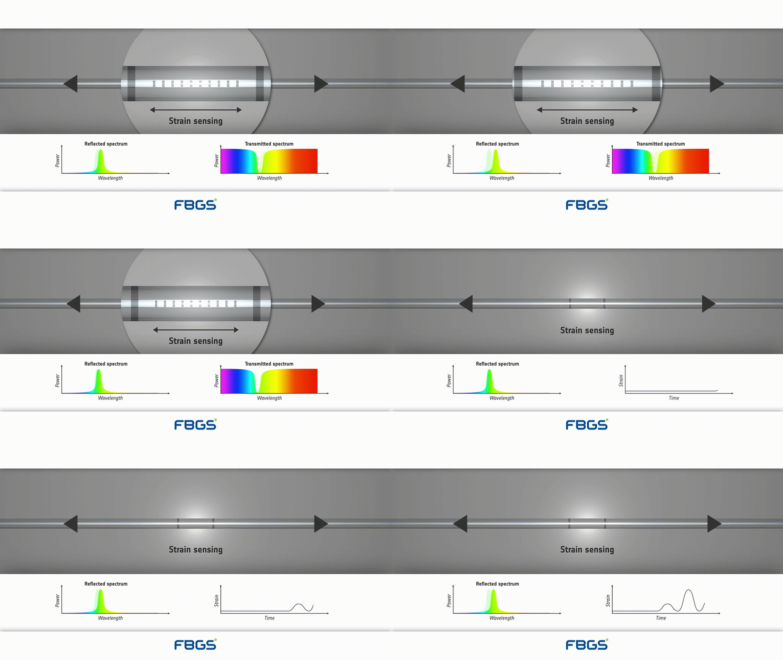
An FBG is a short section of single-mode optical fiber whose core refractive index is modulated periodically over a few millimeters. The grating is written by exposing the core to an interference pattern from a UV laser (or via a photomask or point-by-point inscription). The result is a narrowband mirror embedded inside the fiber: when broadband light propagates down the core, a small band of wavelengths that satisfy the Bragg condition is reflected back while the remainder is transmitted. The process is sketched in Figure 8.
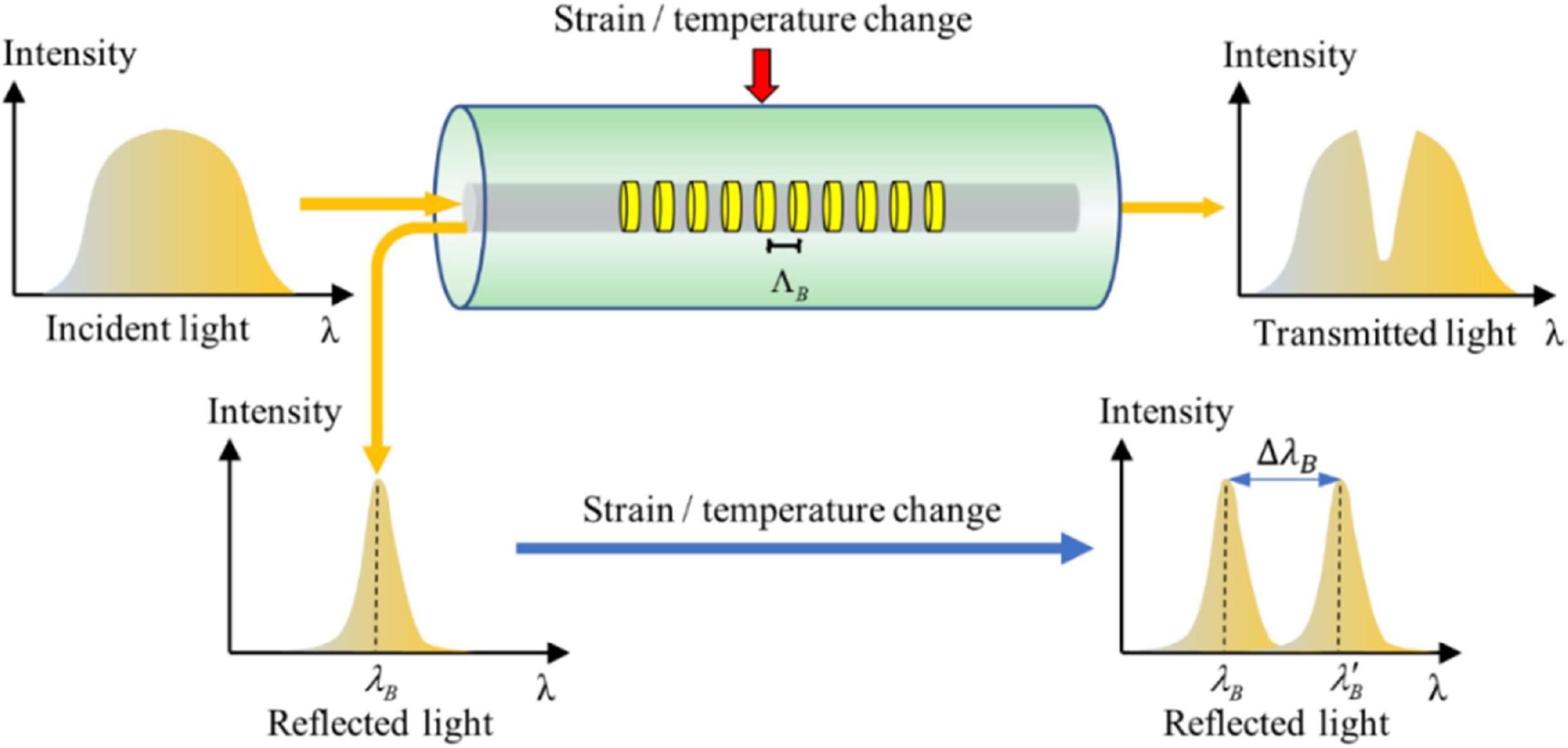
Figure 8:FBG operating concept. A periodic index modulation of period reflects a narrow spectral line at the Bragg wavelength ; applied strain or temperature shifts the reflected peak by .
At the heart of the sensor is the Bragg condition: the wavelength most strongly reflected by a uniform grating of period in a fiber with effective core index is
Any action that changes either the grating pitch or the effective index shifts the reflected wavelength. A convenient differential form follows from (9):
In silica fibers these perturbations are dominated by axial strain and temperature change . Using the photoelastic response of the glass and the thermo-optic and thermal-expansion effects, one obtains the standard FBG sensing law:
where is the effective photoelastic coefficient of the fiber, the coefficient of thermal expansion of the glass, and the thermo-optic coefficient. Equation (11) explains the two essential features of the plots in Figure 9: a load- or temperature-induced shift of the reflected line , and a largely unaltered transmitted spectrum apart from the narrow notch at the reflected wavelength.
5.2Other classes of FOS sensors
Another class is distributed fiber sensing, such as Brillouin or Raman scattering-based systems (e.g. BOTDR, Brillouin Optical Time Domain Reflectometry). These send a pulsed laser through the fiber and measure scattered light returning from every point along the fiber. The spectrum of the backscattered light (Brillouin shift for strain/temperature, Raman for temperature) is analyzed to yield strain or temperature as a continuous function of position along the fiber. The result might be a strain profile every 0.5 m along a fiber that’s several kilometers long, for example. This is powerful for detecting, say, the location of a crack or excessive strain in a bridge deck by seeing a spike in the strain profile.
5.3Capabilities and limits of fiber-optic sensing
Fiber-optic sensors are well suited to bridge monitoring because they move the measurement into the optical domain. Signals are immune to electromagnetic noise, so long runs past traction power, lightning, or radios do not corrupt the data. Single-mode fibers at 1550 nm carry signals over kilometers with little loss, enabling centralized interrogation on long spans or networks. The fiber itself is thin and light, can be surface-bonded or embedded, and, through multiplexing, dozens of FBGs can share one fiber and one interrogator, dramatically reducing cabling. Properly packaged devices are passive at the sensing point (no local power), corrosion-resistant, and durable in wet or hot environments. Interrogators resolve picometer-level wavelength shifts, giving sub-microstrain precision for FBGs and large usable ranges (several thousand ). Distributed methods (Brillouin/Rayleigh) provide continuous profiles over tens of kilometers with meter-scale spatial resolution, useful for long members and liners.
The trade-offs are practical rather than conceptual. Optical interrogators are costly and complex compared with electrical DAQs, especially for high-rate, multi-channel systems. Installation is delicate: glass fibers require careful strain transfer, protection against abrasion and tight bends, and ruggedized routing on site. Because temperature also shifts the optical response, strain measurements need compensation, typically a paired temperature FBG or a thermally compensated package. Distributed sensing sacrifices spatial resolution (0.2–1 m typical) and, depending on the technique, may favor quasi-static measurements; FBGs, by contrast, support kHz dynamics but only at discrete points. As with any sensor, calibration and periodic checks (e.g., known loads or reference FBGs) are required. Net effect: fiber-optic sensors deliver low-noise, long-reach, and densely multiplexed measurements ideal for large bridges, provided the project accepts the higher interrogator cost and the care needed in installation and temperature compensation.
5.4Typical Specs & Performance
A typical FBG strain sensor might have an initial Bragg wavelength around 1550 nm, gauge length ~10 mm, strain range ±5000 , and accuracy of ±1–2 . Temperature cross-sensitivity is often ~10 /°C if uncompensated (meaning a 1 °C temp change mimics 10 strain), so compensation is essential. Sampling rates up to 1 kHz are available on some interrogators for a few FBGs; for many FBGs, rates of 100 Hz or 50 Hz per sensor are common to keep cost reasonable. Distributed Brillouin systems might measure strains with ±20 accuracy, spatial resolution 0.5–1 m, over 10 km length, but at slow update rates (minutes).
6Acoustic Emission Sensors: Detecting Active Damage
Acoustic Emission (AE) monitoring is a technique aimed at capturing the sounds of damage in materials. When cracks grow or fibers break or any rapid micro-structural event occurs in a material under stress, it releases a burst of elastic energy that propagates as stress waves, essentially a high-frequency sound wave traveling through the structure. AE transducers (sensors) are used in SHM to detect these transient elastic waves, with the goal of identifying the onset or progression of cracks and other acute damage mechanisms in bridges. While global vibration sensors (accelerometers) can tell if the structure’s stiffness has changed after damage, AE sensors can catch the moment the damage is occurring. For example, in a steel bridge girder, as a fatigue crack extends a small amount, an AE burst may be emitted; an AE monitoring system can detect this in real-time and even roughly locate the source via triangulation (using multiple sensors). This makes AE a powerful local monitoring tool for active damage.
6.1Principle of Operation
An acoustic emission sensor is essentially a high-frequency vibration sensor (an ultrasonic sensor) that typically uses a piezoelectric element to convert the surface motion (from a passing stress wave) into an electrical signal. AE sensors are usually resonant or broadband piezo transducers that respond to frequencies in the range of ~20 kHz up to 1 MHz (much higher than typical structural vibrations) because crack-related waves have very short durations and high frequency content. When an AE event (like a crack jump) occurs, it generates a stress wave that travels through the material. Upon reaching the sensor location, this wave causes a small displacement/strain on the sensor’s piezo element, generating a voltage spike. The sensor output is an electrical waveform representing the acoustic burst. This is then usually amplified and filtered. Multiple parameters characterize an AE burst: Figure 10 shows a typical waveform from an AE sensor and the standard “hit” features extracted by the detector. The hit begins when the signal first crosses the threshold and ends when it falls back below it; the rise time is the interval from that first crossing to the peak, and the duration is from the first to the last crossing. The amplitude is the peak voltage, while the shaded area (often called MARSE or signal energy) represents the time integral of the rectified, squared waveform over the hit. The pulses produced by the comparator at the bottom illustrate counts, i.e., the number of threshold crossings, which reflect waveform complexity. Together these compact descriptors (amplitude, rise time, duration, counts, and energy) summarize how abrupt and how energetic the event is, and they are the building blocks for noise rejection and mechanism classification in AE monitoring. Acoustic emission signals contain rich information about the damage processes that generate them. Different types of damage mechanisms produce characteristic signal signatures that can be analyzed to understand not only where damage is occurring, but also what type of damage is taking place. For example, Crack growth typically produces signals with sharp rise times and high peak frequencies, reflecting the rapid nature of bond breaking at the molecular level. Fiber breakage in composite materials generates signals with different frequency content and duration compared to matrix cracking. Corrosion processes produce continuous or burst-type emissions with lower frequencies and longer durations. Advanced pattern recognition techniques are increasingly used to classify different types of damage based on their acoustic emission signatures, enabling automated assessment of damage severity and growth rates.
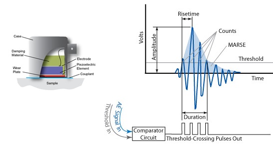
Figure 10:Typical acoustic-emission sensor structure and its signal type [Source].
6.2Source location by time-difference of arrival (TDOA)
A critical aspect of AE in structures is source location. By using an array of AE sensors, one can triangulate the source of the emission, similar to how microphones can locate a sound source. If a crack emits a wave, it will reach the nearest sensor slightly before the farther ones. By measuring the difference in arrival times (time of flight) between sensors, and knowing the wave speed in the material (usually the transverse wave speed for the dominant mode, on the order of 3 km/s in steel or 1.5 km/s in concrete), the location of the crack can be estimated. This requires accurate timing and typically a high sampling rate to capture timing differences on the order of microseconds. For example, when two sensors are mounted a known distance apart along a member, a transient from a flaw reaches one sensor earlier than the other. If is the measured arrival-time difference (second minus first) and is the relevant wave velocity for the material and mode (e.g., longitudinal in a rod, Lamb-wave in a plate), the one-dimensional source position measured from the first-hit sensor is
The geometry and waveforms are illustrated in Figure 11: the same event produces two similar bursts shifted in time; the sign and magnitude of determine which side and how far the source lies. In practice, is obtained from calibration shots (e.g., Hsu–Nielsen pencil-lead breaks) because real structures are dispersive and boundary-dependent. For plates and complex geometries, arrays with three or more sensors extend the idea to 2-D/3-D triangulation.
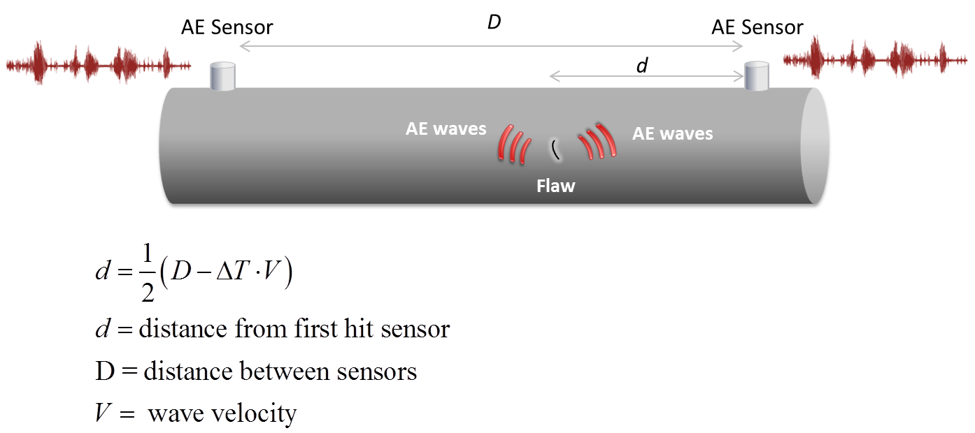
Figure 11:Linear AE source location on a prismatic member using two sensors [Source].
6.3Strengths and limitations of acoustic emission (AE)
AE’s distinctive value is timeliness: it listens for stress-wave bursts emitted the moment damage nucleates or grows, providing real-time surveillance of active cracks, fretting, or wire breaks. Because stress waves propagate metres through steel and concrete, a small array can cover large regions, making AE cost-effective where crack locations are uncertain. The method is passive and highly sensitive, able to detect micro-events that do not yet alter strains or global vibration, and can be configured to issue immediate alarms. Patterns in the hits (rates, spectra, rise times) often help discriminate mechanisms such as rubbing versus brittle fracture, focusing inspection where progression is actually occurring.
The trade-offs are practical. Bridges are acoustically busy, so background noise can trigger false positives or mask weak events; mitigation relies on band-pass filtering, adaptive thresholds, and sensor-to-sensor correlation. Attenuation and scattering, especially in concrete and across joints, limit the area a sensor can reliably cover and can blur source localization to a region rather than a point. Active periods generate large data volumes that require real-time feature extraction and robust storage. AE is also qualitative about capacity: it indicates that damage is occurring, not its exact size, so follow-up NDE (e.g., UT) is often needed. Finally, successful deployment demands careful coupling and configuration (sensor type and frequency, thresholds, calibration of wave speeds) and experienced interpretation. When these considerations are addressed, AE is a powerful complement to strain and vibration monitoring, offering early warning and efficient coverage of complex bridge details.
6.4Typical Specs & Performance
AE transducers often have resonant frequencies in the 100–300 kHz range (like a common resonant sensor at 150 kHz) since many crack emissions in metal peak around that range. Some are broadband sensors (e.g. 50–400 kHz useful range) for more general use. Sensitivity is usually given in decibels (dB) referenced to some velocity or pressure, but in practice an AE sensor can detect displacements on the order of nanometers. The instrumentation (preamplifiers) typically have gain settings (20, 40, 60 dB, etc.) and band-pass filters to focus on the desired frequency band (to cut out low-frequency noise and very high-frequency electronic noise). AE systems often sample the waveforms at 1–5 MHz with 12- or 16-bit ADCs to get a detailed shape. Because storing full waveforms continuously would be huge, they often operate in a trigger mode: when the signal crosses a threshold, a window of the waveform is recorded (e.g. 200 µs before and 1000 µs after threshold, capturing the burst). This is then saved and basic features are extracted.
In steel, an AE sensor might reliably detect a 0.1 mm crack growth event from several meters away, whereas in concrete, the range might be shorter (because concrete, with its aggregate, heavily attenuates high-frequency waves). The speed of wave used for timing is often around 5000 m/s for longitudinal waves in steel, 3000 m/s for extensional waves, or ~3000 m/s in concrete (depending on mode and material). Source location accuracy can be within ±0.5 m if well calibrated.
7Vision-Based Sensors
Vision-based sensing refers to using cameras and image processing techniques to monitor structural behavior. They can measure displacements, strains, and detect surface damage (like cracks or spalls) from a distance. The ability to remotely monitor a bridge using cameras is extremely attractive: one can measure displacement or strain at many points without installing physical sensors, simply by processing the images or video frames of the structure. For instance, cameras have been used to track the deflection of a bridge span under load by focusing on targets or natural features on the bridge and computing their movement in the video frames. Vision-based methods can also automatically detect cracks, corrosion spots, or other surface anomalies on bridge components. This can greatly augment or even partially automate traditional visual inspections. The motivation is two-fold: (1) practicality, since it is often easier to set up a camera on a tripod or mount than to physically install multiple contact sensors, and (2) rich information, since a single camera view can capture the motion of many points at once (full-field measurement), something that would require dozens of accelerometers or LVDTs to achieve. Given recent advances in high-speed cameras and computer vision algorithms, vision-based SHM has moved from conceptual research to real-world application on bridges, demonstrating accurate measurement of dynamic displacements in the order of 0.01–1 mm from tens of meters away, as well as reliable crack detection using machine learning on images.
7.1Principle of Operation
At the core, vision-based sensing involves filming or photographing the structure and then extracting quantitative measurements from the imagery. For displacement or vibration measurement, the usual approach is to identify feature points on the structure (either natural texture, edges, or attached markers) and track their positions in each frame of a video. By calibrating the camera view (knowing the scale of pixels to real-world units, via a calibration target or known dimensions on the structure), the pixel movements can be converted to physical displacements. For example, if a bridge girder’s bottom edge is visible in the camera, one can track that edge’s vertical position frame by frame to get the deflection time history. Techniques like digital image correlation (DIC) or optical flow can be used to track deformations over a region (full-field deformation/strain). Simpler approaches might use target tracking, for example placing high-contrast targets (like QR codes or colored dots) on the structure and using the camera to track those dot positions.
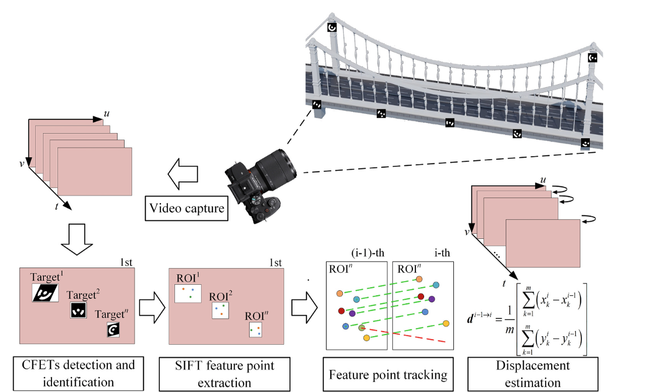
Figure 12:Vision-based bridge displacement measurement process [Source].
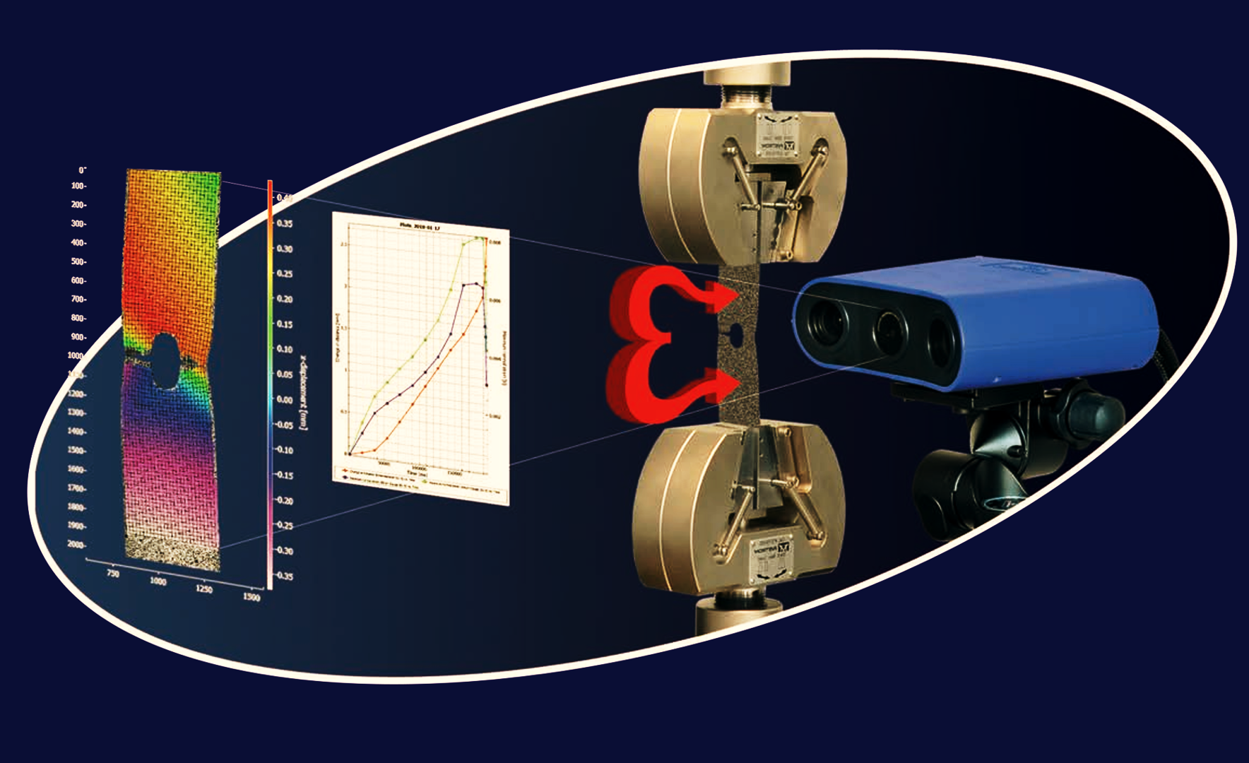
Figure 13:Vision-based full-field strain measurement [Source].
Another key step is camera calibration: determining the intrinsic parameters (focal length, lens distortion) and extrinsic parameters (orientation and position relative to structure). Calibration allows one to map image coordinates to real-world coordinates. In practice, if the camera is viewing the structure at an angle, one might simplify by aligning the optical axis normal to the plane of motion so that a pixel shift corresponds linearly to displacement (or use a homography transform for planar movement). Equation-wise, one often uses the pinhole camera model:
which relates a 3D point on the structure to its image pixel . Here is the camera intrinsic matrix and are rotation and translation. By simplifying this (for small deflections, or known planar geometry), one can derive a scale factor between pixel movement and actual displacement. For example, if an object of known length spans pixels in the image, the scale is per pixel. Thus a measured deflection of pixels corresponds to in real units (assuming deflection in the same plane as the reference object). This is a basic calibration approach. Modern techniques often involve performing a one-time calibration using a checkerboard or known markers to compute all parameters, then any pixel measurements can be scaled (accounting for perspective and distortion).
For damage detection like crack finding, computer vision algorithms treat it as an image recognition task. High-res images of the structure are captured, and either image processing (edge detection, filtering) or machine learning (deep convolutional neural networks trained to spot cracks) are applied to locate and quantify defects. Figure 14 shows a typical computer-vision workflow for crack analysis on concrete. Panel (a) is the raw image; (b) a tile-based classifier highlights crack-likely patches (gold); (c) an object detector returns bounding boxes around crack regions (red); and (d) semantic segmentation produces a pixel-level mask (white) that can be converted to length/width after camera calibration. In practice, detection is used to screen large areas quickly, while segmentation provides the geometry needed for measurement and trend tracking.
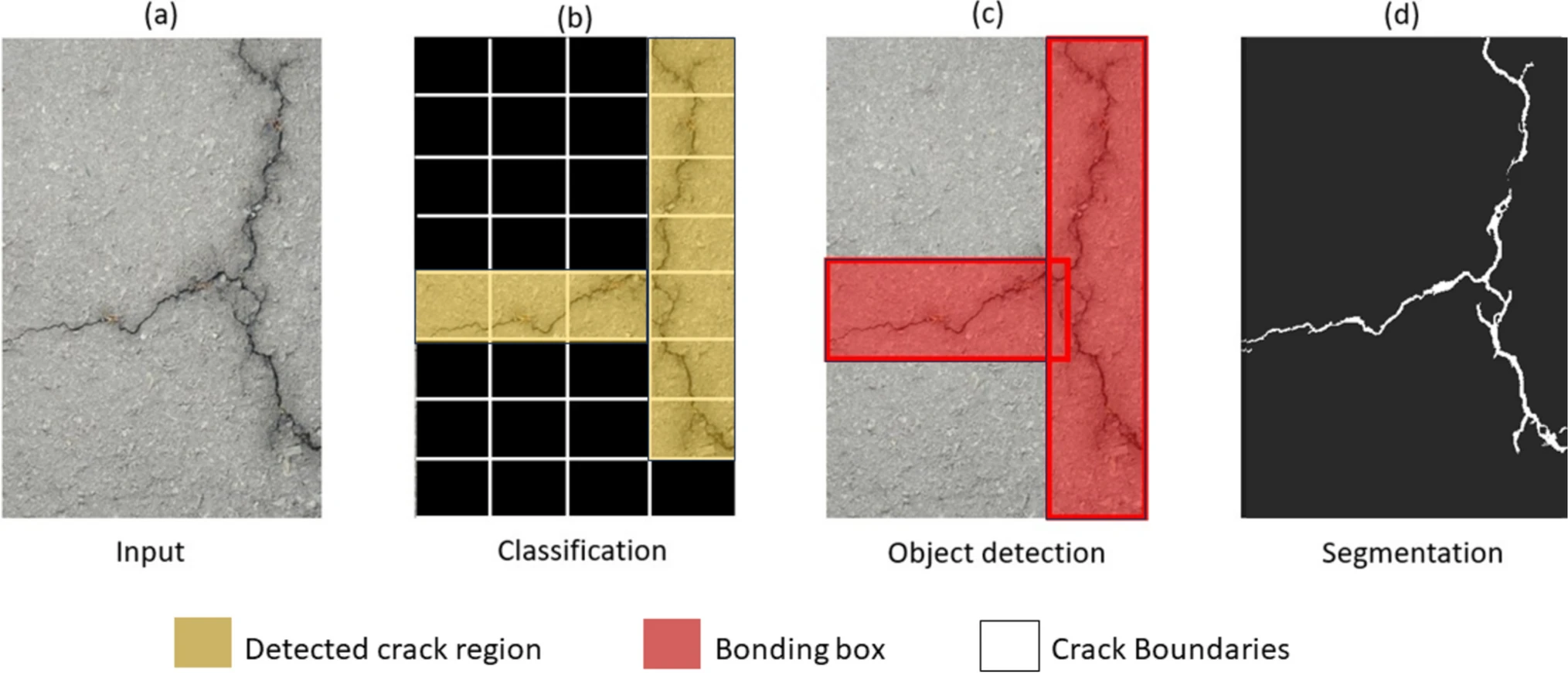
Figure 14:Vision-based crack analysis pipeline: (a) input image, (b) patch classification (gold tiles), (c) object detection (red boxes), and (d) segmentation (white crack mask) for quantitative measurement.
7.2Limitations of vision-based sensors
Vision systems are highly sensitive to the scene. Changing sunlight, headlight glare, rain, fog, and night conditions alter contrast and can break feature tracking; maintaining consistent illumination often requires auxiliary lighting or infrared/thermal cameras. Measurements also rely on a stable, well-calibrated camera: any motion of the mount shows up as false displacement, lens distortion skews geometry, and temperature drift can invalidate calibration. Because the method is line-of-sight, occlusions from vehicles or equipment cause data dropouts, and out-of-plane motion or camera jitter can bias in-plane displacement unless a fixed reference or dual-camera compensation is used.
Performance is bounded by resolution and frame rate. At long standoff distances, small structural motions may move a feature by only a fraction of a pixel; while sub-pixel methods help, accuracy degrades as pixels per target shrink. Standard video (30–60 fps) cannot capture higher-frequency modes or short transients; high-speed cameras improve bandwidth but at the cost of resolution, data volume, and expense. Finally, robust vision SHM needs heavy computation and careful algorithms to avoid false positives (e.g., stains flagged as cracks) and to convert pixels to physical units; complex structures often require multiple viewpoints, careful placement, and periodic re-calibration to keep results reliable.
7.3Typical Specs & Performance
A typical setup for measuring bridge deflection might use a 1080p or 4K resolution camera with a telephoto lens from, say, 50 m away, achieving a scale like 1 pixel = 0.5 mm. If the bridge deflects 5 mm, that’s a 10 pixel movement, easily detectable. The precision after sub-pixel interpolation might be 0.1 pixel or better, so ~0.05 mm, which is very good. Higher resolution (e.g. 4K, 8K cameras) can improve that further or allow coverage of larger area with the same resolution per target. Frame rates of 30–60 fps typically handle normal traffic-induced vibrations (0–10 Hz) adequately. For capturing modal frequencies up to, say, 20 Hz, a 50–60 fps camera is advisable. Some researchers use 120 fps (in reduced resolution modes) to capture up to 50–60 Hz modes if needed.
In crack detection, a high-res still camera (20+ megapixel) might detect cracks on the order of 0.1 mm width at a few meters distance. From a drone or distance, one might detect ~1 mm cracks at best with current tech. So for fine cracks, close-up inspection is still needed, but the medium to large cracks can be found via imaging.
8Smartphone-Based Sensing
The ubiquity of smartphones, packed with sensors and network connectivity, has opened a low-cost pathway to crowdsourced SHM. Modern smartphones contain MEMS accelerometers, gyroscopes, magnetometers, GPS, cameras, and more, effectively making them multi-sensor nodes that people carry everywhere. Researchers have recognized that these can be used for structural monitoring in two primary ways: (1) Fixed deployment: attaching or placing smartphones on a structure as makeshift wireless sensors (e.g., strapping a smartphone to a bridge railing to record vibrations), and (2) Mobile sensing: using smartphones in moving vehicles (or carried by pedestrians) crossing a bridge to gather vibration data of that bridge. Smartphone-based monitoring applications span a broad spectrum of structural assessment tasks, from rapid post-earthquake damage evaluation to long-term monitoring of critical infrastructure. Figure 15 illustrates the diverse applications where smartphone sensing has proven effective.
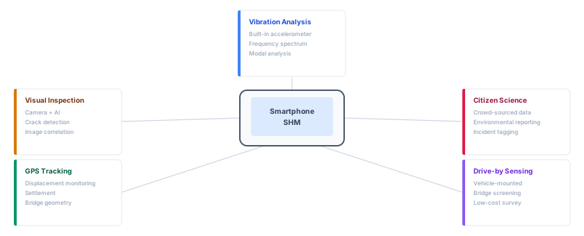
Figure 15:Overview of smartphone applications in different fields.
8.1Principle of Operation
Using smartphones for SHM involves creative use of their internal sensors. The primary sensor used is the accelerometer. Smartphones have triaxial MEMS accelerometers (commonly used for screen orientation etc.) that can sample typically up to 100 Hz or more (some up to 200–400 Hz on high-performance modes). To measure a bridge’s vibration, one can either: place the phone stationary on the structure (and record acceleration due to ambient or forced vibrations), or let the phone measure from within a moving vehicle. In the stationary case, the phone is effectively a self-contained seismometer; many apps have been developed to record accelerations (some even target structural monitoring). The quality of data can be decent: although phone accelerometers have more noise and lower resolution than dedicated ones, they can capture the dominant bridge frequencies, which are usually under ~20 Hz.
In the moving vehicle case, as a car/truck goes over a bridge, both the bridge and vehicle vibrate. The phone inside measures a convolution of vehicle and bridge dynamics. Various approaches (filtering, system identification techniques) have been proposed to extract the bridge’s frequency from these measurements, essentially trying to separate the vehicle’s own bounce frequency and the road roughness effects to isolate the bridge’s influence. It’s challenging but studies (some cited in the smartphone literature) have indeed extracted bridge natural frequencies from drive-by data, and even changes in them due to damage. Another smartphone sensor, the gyroscope, can measure rotational motion (which could be used to sense inclination changes or torsional modes of a bridge if the phone is positioned appropriately). The GPS in phones, while not precise enough for small deflection measurement on a single pass (GPS has ~3-5 m accuracy in position), can provide velocity or acceleration through differentiation at low frequencies or be used to time-synchronize data across multiple phones. Also, if many passes are averaged, GPS could detect frequency content (some research attempts to use the slight vertical accelerations detected in GPS when going over a bridge).
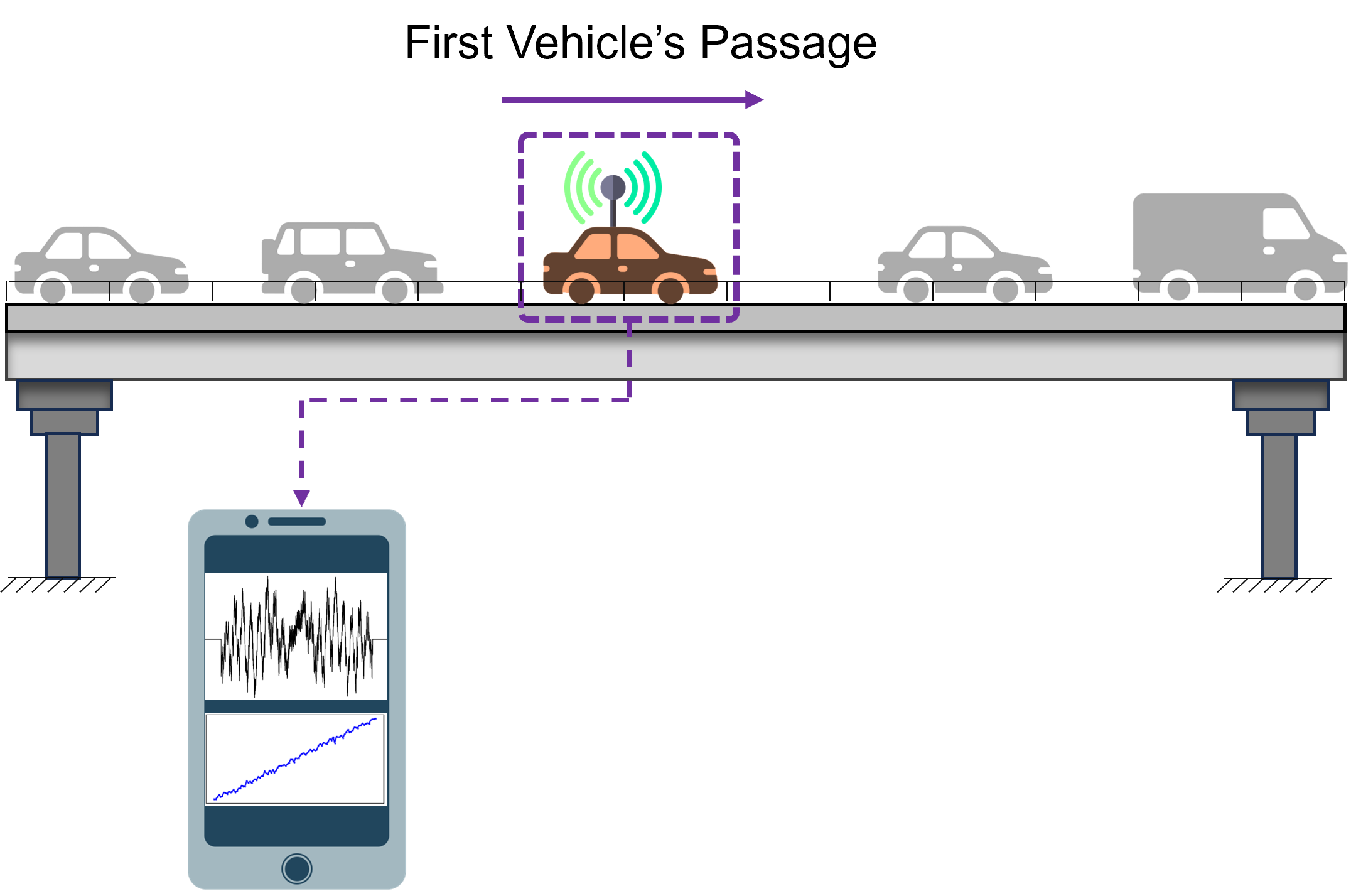
Figure 16:Mobile sensing using smartphones.
Smartphone cameras can also play a role: for instance, one could record a bridge’s motion via the phone camera (a simplified vision-based method) or use a phone’s camera for crack detection by taking pictures (crowdsourced imagery of bridges). However, camera usage is limited by needing vantage points; still, a phone camera could potentially measure the deflection of a nearby small bridge by video (like on short footbridges).
The process typically involves an app or software on the phone that records the sensor data, possibly processes it (e.g., computing an FFT of the acceleration), and then uploads results to a server. One app you can try is shown below, programmed by the authors. A professional-grade alternative is phyphox, a reliable and complete app that you can download and test for free at https://
🔬 Lab Tool: AccelTracker Pro
Features:
Real-time 3-axis acceleration monitoring
Configurable sampling rate (25/50/75/100 Hz)
Interactive charts with zoom/pan
Excel export with metadata
Professional data visualization
8.2Typical performance
The following table summarizes what you can reasonably expect from phone-class sensors when used for quick SHM checks. Values are indicative, since handset models and OS APIs differ, and power numbers refer to the sensor (not the whole phone). In practice, accelerometer/gyroscope streams are commonly limited to 50–200 Hz, microphones to 44.1–48 kHz, GPS to 1–10 Hz, and cameras to 30–60 fps (higher with trade-offs). Scene resolution for vision depends strongly on optics and distance; the example given assumes a tele/standard lens with typical fields of view.
Table 3:Smartphone sensor capabilities, power, and SHM application notes
| Sensor type | Typical range | Resolution / sampling | Power (sensor) | SHM uses | Key limitations |
|---|---|---|---|---|---|
| Accelerometer | ±2–±16 g | ~0.01–0.1 m/s² ; 50–200 Hz | ~10 µW | Vibration screening; modal frequency ID | Noise floor, orientation dependence, OS filtering |
| Gyroscope | ±250–±2000 °/s | ~0.01 °/s ; 50–200 Hz | ~5 µW | Rotation/tilt, torsional modes (screening) | Bias drift, temperature sensitivity |
| Magnetometer | ±1200 µT | ~0.1 µT ; 10–50 Hz | ~15 µW | Heading/reference, coarse orientation | Magnetic interference, hard/soft-iron errors |
| GPS/GNSS | Global | 1–5 m (civil); 1–10 Hz | ~100 mW | Geotagging, speed, rough displacement | Multipath; limited accuracy for small motions |
| Camera | 1080p–4K video, 12 MP+ stills | Scene-dependent (e.g., ~0.2–1.0 mm/px at ~10 m) ; 30–60 fps (higher on HS modes) | ~500 mW (recording) | Visual inspection, crack imaging, DIC/optical tracking | Lighting/weather, line-of-sight, calibration, data size |
| Microphone | 20 Hz–20 kHz | 16–24-bit ; 44.1–48 kHz | ~50 mW (recording) | Acoustic/vibro-acoustic events, impact tests | Background noise, placement sensitivity |
| Barometer | 300–1100 hPa | ~0.1 hPa ; 1–10 Hz | ~1 µW | Altitude/pressure context, temperature-comp. aids | Temperature drift; enclosure effects |
8.3Limitations of smartphone-based sensing
Smartphones are not precision instruments. Their accelerometers have a relatively high noise floor, limited dynamic range, and often apply undocumented filtering in the operating system. Access to truly raw data can be difficult, and readings vary across models and even units; bias, scale, and temperature drift are common. Sampling rates are capped (often ≤100–200 Hz) and timestamps can jitter, which complicates spectral analysis and any attempt to synchronize multiple phones. Small bridge responses, such as millig-level vibrations or subtle frequency shifts, can sit at or below these limits.
Field use adds further constraints. Mounting is rarely rigid; phone motion or orientation changes contaminate measurements, and vehicle crossings mix bridge dynamics with suspension and road-roughness effects, shortening usable record lengths and requiring heavy post-processing. Long-term deployments face power, weather, and security issues; crowdsourced schemes depend on voluntary participation and raise privacy and data-governance questions. In practice, phones are best for screening and quick checks (e.g., rough estimates of dominant frequencies). For diagnostics that rely on low-level responses, precise timing, or repeatable calibration, dedicated sensors and DAQ remain the more reliable option.
9Data Acquisition Systems (DAQ)
The data acquisition system is the bridge between sensors and analysis. It must accept different input types, sample with accurate timing, and move data reliably to storage and visualization, often for months in the field. The figure below summarizes the core building blocks common to SHM deployments.
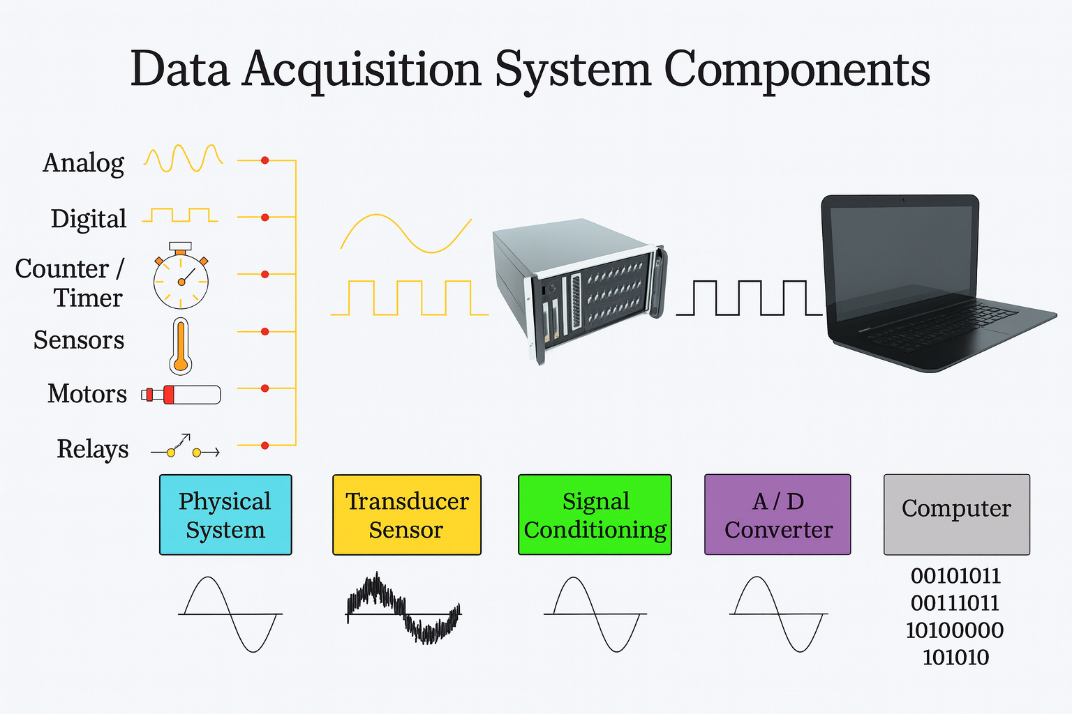
Figure 17:Core components of a data acquisition system [Source].
As shown in Figure 17, each block has a specific role:
Transducer/Sensor. Converts a physical quantity (strain, acceleration, temperature, displacement) into an electrical signal. Outputs may be continuous voltages/currents or discrete events and pulses.
Signal conditioning. Prepares the sensor output for digitization: excitation and bridge completion, amplification to match ADC ranges, anti‑alias filtering, multiplexing when channels are shared, and electrical isolation to avoid ground loops and protect equipment.
A/D conversion and timing. Samples the conditioned signal and produces digital data. For SHM, 16–24‑bit converters provide the dynamic range to capture both ambient and traffic‑induced responses. Systems may use simultaneous sampling or fast multiplexing; in both cases a stable hardware clock governs the sample rate. For distributed systems, GPS or IEEE‑1588/PTP can supply a common time base so measurements align across nodes.
Host computer and software. Interfaces with the DAQ (USB, Ethernet, or embedded controller), buffers and logs data, and supports visualization and quality checks. Acquisition software manages triggers, timestamps, and metadata so records can be traced to the exact sensor configuration.
10Wireless/IoT Sensor Nodes
Wiring an array of sensors across a large bridge can be labor-intensive, costly, and sometimes impractical. Wireless sensor nodes (often called smart sensors or IoT nodes when they include on-board processing) offer a solution by eliminating long cable runs and allowing flexible deployments of sensors. In SHM, wireless sensor networks (WSNs) have become increasingly popular for instrumenting bridges because they drastically reduce installation and maintenance costs compared to traditional tethered systems. For aging bridges that need retrofitted monitoring, wireless nodes can be attached with minimal intrusion and without needing to route cables through traffic or structures. Wireless nodes are typically battery-powered devices that integrate one or more sensors (e.g. an accelerometer, strain gauge, thermometer), a local processor, storage, and a radio transmitter. They collect data from the sensor, do some processing (possibly filtering or compressing data), and then transmit the data (or summary) to a central gateway or base station. In the context of IoT (Internet of Things), modern SHM wireless nodes can even send data to the cloud or allow remote monitoring in real time.
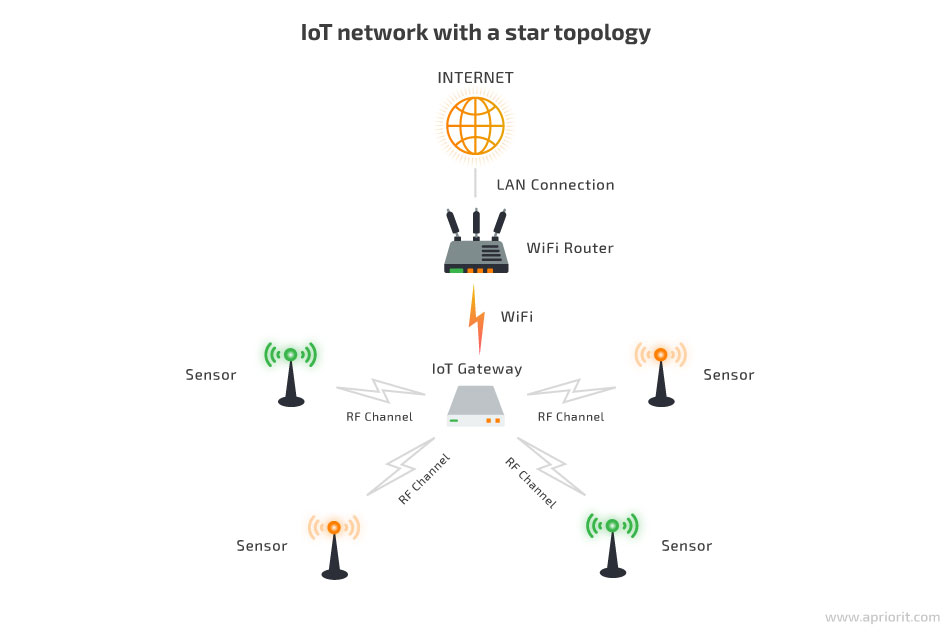
Figure 18:Typical Wireless/IoT node architecture [Source].
10.1System Concept
A wireless SHM node typically consists of several components: (1) Sensors (could be built-in, like a MEMS accelerometer or external like a strain gauge that can be attached), (2) Analog-to-digital converters (ADC) to digitize sensor signals (often 12-bit or 16-bit resolution), (3) a microcontroller or processor to manage sensor reading and possibly perform computations, (4) a wireless radio transceiver (often using standards like Zigbee/IEEE 802.15.4, Wi-Fi, or custom protocols), and (5) a power source, usually a battery (sometimes with solar or vibration energy harvesters to extend life). These nodes communicate either directly to a central gateway or in an ad-hoc mesh network where data hops from node to node until reaching a gateway. The gateway then relays data to a server or local storage for analysis.
Each node can be considered a miniature DAQ system on its own, just untethered. For example, a wireless accelerometer node might sample acceleration at 200 Hz, compute FFT onboard, and wirelessly send the FFT peaks rather than the entire time history, to conserve power and bandwidth. More advanced nodes synchronize with each other via wireless time-sync protocols, so that data from different nodes is time-aligned (important for modal analysis or triangulating events). Table 4 summarizes pros and cons.
Table 4:Wireless SHM Sensor Nodes: Pros and Cons
| Advantages | Disadvantages |
|---|---|
| No long cables needed (lower install cost) | Battery-powered: limited life, maintenance to replace/charge |
| Scalable to many nodes (easy to add sensors) | Wireless communication can be unreliable (signal loss, interference) |
| Can cover large areas: mesh networking spans entire bridge | Bandwidth constraints: may not stream high-rate data from many nodes |
| On-board processing reduces data load | Time sync is complex: slight desynchronization possible between nodes |
| Easy remote access to data (if networked) | Environmental exposure of electronics (need ruggedization) |
| Supports multi-sensor fusion in one node (e.g., accel + temp) | Initial setup of network and calibration is needed (more complex system) |
| Adaptive: nodes can be moved or re-tasked easily | Potential cybersecurity concerns (ensure data integrity over wireless) |
10.2DAQ Considerations
In a wireless node, the DAQ is integrated. Key considerations include the ADC resolution and sampling rate (often a trade-off with power, since higher-bit ADCs and faster sampling use more power). Many platforms use 12-bit ADCs to save power, which can be adequate, though some newer ones use 16 or 24-bit for strain measurements. For example, a typical wireless strain node might sample at 100 Hz with a 16-bit ADC and store data locally, then transmit either the raw data or computed values (like damage indices) at intervals. Because continuous streaming is costly on battery, some systems employ event-triggered acquisition: e.g., continuously monitor acceleration at low power; if a trigger threshold is exceeded, start recording at higher sampling and send that snippet. This way you capture only interesting events (like unusually high vibrations from maybe a blast or a vehicle impact).
To maintain synchronization, wireless nodes often exchange periodic sync messages. Some DAQ architectures will timestamp data at the node with respect to a global clock (maybe GPS or the gateway’s clock), ensuring data alignment when merged.
10.3Performance vs. wired
Numerous validation experiments have been done. Generally, for low-frequency structural monitoring, wireless systems can match wired performance in terms of data quality. The differences might appear in slightly higher noise floor (due to lower ADC resolution or radio interference) or occasional data gaps. But for extracting modal frequencies or tracking large strain changes, they are effective. If high fidelity is needed (e.g. detecting small damping changes), the noise or sync issues in wireless might impede that analysis.
11Sensor Comparison and Selection Criteria
The selection of appropriate sensor technologies for a specific bridge monitoring application requires careful consideration of multiple factors including measurement requirements, environmental conditions, budget constraints, and long-term maintenance needs. This section provides initial guidance for making informed sensor selection decisions.
11.1Systematic Performance Comparison
A systematic comparison of sensor technologies requires evaluation across multiple dimensions including cost, coverage, sensitivity, bandwidth, install complexity, and durability against your monitoring objective and site constraints. The following radar view summarizes the key characteristics of major sensor technologies used in bridge monitoring:
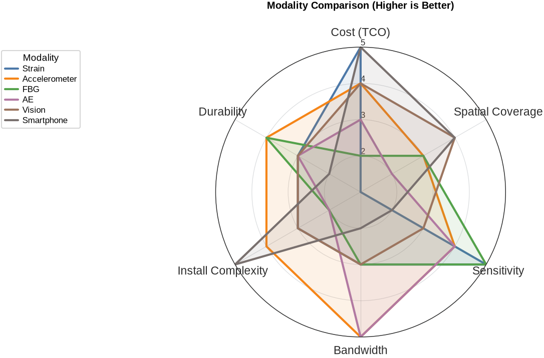
This comparison reveals that no single sensor technology is optimal for all applications. Instead, effective monitoring systems typically employ combinations of technologies that complement each other’s strengths and compensate for individual limitations.
11.2Decision Framework and Selection Process
The sensor selection process should follow a systematic framework that considers the specific requirements and constraints of each monitoring application. The following figure presents a decision tree that guides this selection process.
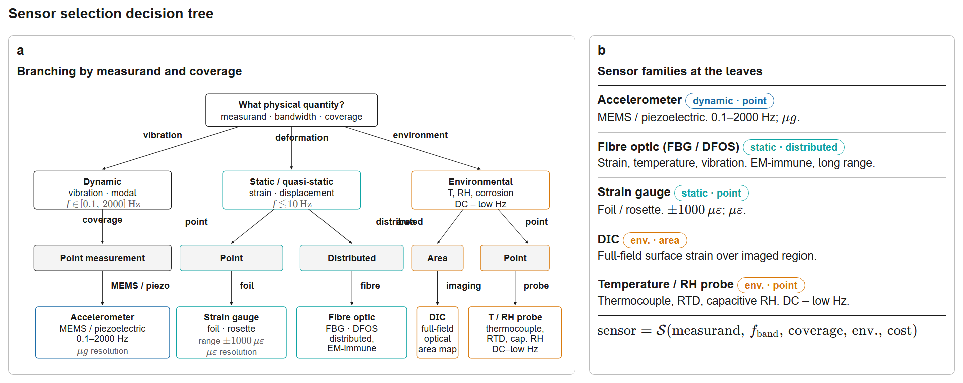
Figure 20:Decision tree for sensor selection in bridge SHM applications, considering primary measurement requirements (frequency range, coverage) and secondary practical constraints.
The decision framework illustrated in Figure 20 provides a systematic approach to sensor selection that considers both technical requirements and practical constraints. The process begins with identifying the primary measurement parameter, then branches into specific technology choices based on coverage requirements, frequency ranges, and measurement approaches.
Primary Parameter Selection forms the foundation of the decision process. Strain measurements are essential for understanding stress distributions and identifying locations of high stress concentration. Vibration measurements provide information about structural dynamics and can reveal changes in stiffness or boundary conditions. Displacement measurements quantify overall structural deformation and are particularly important for serviceability assessment.
Secondary Criteria often prove decisive in the final sensor selection. Budget constraints significantly influence technology choices, with smartphone-based systems offering very low-cost solutions for temporary monitoring, while high-precision piezoelectric accelerometers represent significant investments justified only for critical applications requiring exceptional accuracy.
Environmental considerations play a crucial role in sensor longevity and measurement reliability. Marine environments with salt spray exposure favor fiber optic sensors due to their inherent corrosion resistance, while standard atmospheric conditions allow use of properly protected conventional sensors.
Installation access affects both initial deployment costs and long-term maintenance requirements. Bridges with limited access or historical significance may favor non-contact measurement approaches, while structures with good access can benefit from the typically superior accuracy of contact-based sensors.
Monitoring duration influences both sensor selection and system design. Long-term permanent monitoring systems justify investment in robust, stable technologies with proven longevity, while short-term monitoring for construction or load testing applications may prioritize ease of installation and lower initial cost over long-term stability.
12Installation and Environmental Considerations
Bridge sensors must survive in some of the most challenging environments encountered in engineering applications. Developing effective protection strategies requires understanding the specific threats present in bridge environments and implementing appropriate countermeasures.
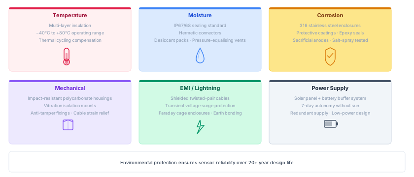
Figure 21:Environmental protection strategies for bridge monitoring sensors, addressing the major threats encountered in outdoor installations.
The protection strategies illustrated in Figure 21 address the primary environmental threats that can compromise sensor performance and longevity. Each protection system must be designed for the specific environmental conditions at the installation site, considering factors such as proximity to salt water, industrial pollution levels, temperature extremes, and lightning exposure.
Temperature Protection must address both the absolute temperature range and the rate of temperature change. Bridge sensors may experience temperature swings of 80°C or more between winter and summer extremes, with daily cycles of 20-40°C. These thermal cycles create mechanical stress in sensor components and connections, potentially leading to drift or failure. Multi-layer insulation systems, thermal barriers, and component selection for extended temperature ranges all contribute to reliable operation.
Moisture Control represents one of the most critical protection requirements. Even small amounts of moisture ingress can cause corrosion, electrical leakage, and measurement drift. Hermetic sealing using O-rings, gaskets, and welded enclosures provides the primary barrier, while desiccant systems handle any moisture that does penetrate the enclosure. Pressure equalization systems prevent seal failure due to thermal expansion and contraction of enclosed air.
Corrosion Prevention requires both material selection and active protection systems. Stainless steel alloys (particularly 316 grade) provide excellent corrosion resistance for most applications, while specialized coatings offer additional protection in severe environments. Sacrificial anodes can provide cathodic protection for metallic components, while proper electrical isolation prevents galvanic corrosion between dissimilar metals.
13Future Trends and Emerging Technologies
The field of structural health monitoring is experiencing rapid evolution driven by advances in multiple technology domains. Understanding these trends is essential for making informed decisions about current system implementations while preparing for future capabilities.
13.1Technology Integration and Intelligence
The future of bridge monitoring sensors lies not in individual technological advances, but in the intelligent integration of multiple sensing modalities, advanced materials, and artificial intelligence.
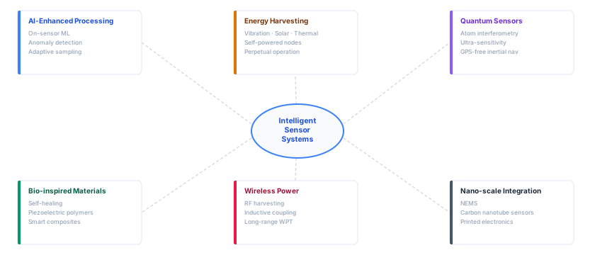
Figure 22:Emerging trends in sensor technology for structural health monitoring, showing the convergence of artificial intelligence, advanced materials, and quantum technologies.
The technological convergence illustrated in Figure 22 represents a fundamental shift from passive sensing devices to intelligent, adaptive monitoring systems. These future systems will possess capabilities that far exceed current technologies, enabling new approaches to structural assessment and maintenance.
AI-Enhanced Processing will transform sensors from simple transducers into intelligent nodes capable of real-time analysis, pattern recognition, and decision-making. Edge computing capabilities will enable sensors to process data locally, reducing communication bandwidth requirements while providing immediate alerts for critical conditions. Machine learning algorithms embedded in sensor nodes will enable adaptive sampling strategies that focus measurement resources on the most informative data while reducing power consumption during periods of low activity.
Energy Harvesting Technologies will eliminate the need for battery replacement and grid power connections, enabling truly autonomous sensor nodes. Advanced piezoelectric materials will convert structural vibrations into electrical energy, while high-efficiency photovoltaic cells and thermoelectric generators will harvest energy from environmental sources. Energy storage systems using supercapacitors and advanced battery technologies will provide reliable power during periods of low energy availability.
Quantum Sensing Technologies promise measurement capabilities orders of magnitude more sensitive than current sensors. Quantum gravimeters can detect changes in local gravitational fields caused by structural density variations, enabling detection of internal damage or structural changes without direct contact. Quantum-enhanced accelerometers and strain sensors will provide unprecedented precision for detecting subtle changes in structural behavior.
14Exercises
Solution to Exercise 1 #
Recommended System Architecture:
Primary Strain Monitoring:
20 electrical strain gauges at critical cable anchorages and deck sections: $25,000
4 distributed FBG arrays (150m each) along main girders: $120,000
Rationale: FBG sensors chosen for marine environment corrosion resistance and distributed coverage
Dynamic Response Monitoring:
12 MEMS accelerometers in weatherproof enclosures: $15,000
4 high-precision piezoelectric accelerometers at key locations: $20,000
Rationale: Hybrid approach balances cost and performance for different analysis needs
Displacement Monitoring:
6 GPS RTK stations for absolute positioning: $45,000
Rationale: Essential for long-term settlement and thermal movement tracking
Environmental Monitoring:
3 weather stations (wind, temperature, humidity): $18,000
Rationale: Critical for data interpretation and environmental compensation
Data Acquisition and Infrastructure:
Ruggedized DAQ system with cellular communication: $80,000
Solar power systems with battery backup: $25,000
Installation, commissioning, and 5-year support: $47,000
Total System Cost: $395,000
Risk Mitigation:
Phased implementation starting with most critical sensors
Redundant measurements at key locations
Modular design allowing technology upgrades
Solution to Exercise 2 #
(a) Using the definition of gauge factor, , we solve for : So the resistance increases by about 0.35 Ω (since tension causes a positive ΔR).
(b) In a quarter-bridge, the approximate output fraction for a small ΔR is (because only one of the four resistors changes, so the bridge becomes slightly unbalanced). Thus the output voltage . The denominator , so In other words, about 1.3 mV change. This is a very small signal, illustrating why amplification is required for strain gauge measurements.
Solution to Exercise 3 #
(a) Advantage 1: Electromagnetic immunity and low signal loss: Fiber-optic sensors are immune to EMI and can transmit signals over kilometers without significant loss. This makes them ideal for bridges in electrically noisy environments or for long-span bridges where long cable runs are needed. Advantage 2: Ability to multiplex many sensors on one fiber: Using Fiber Bragg Gratings or distributed sensing, multiple measurement points can share a single fiber line. This greatly reduces cabling complexity and allows dense sensor coverage (many points of strain or temperature) with minimal hardware. Other possible advantages students might mention: small size and ease of embedding in materials, and excellent long-term stability and corrosion resistance of fiber sensors. (b) One significant challenge is the cost/complexity of the optical interrogator equipment and associated installation. The interrogators (the devices that send/receive light and interpret the signals) are relatively expensive and require technical expertise to set up. Another practical limitation: fragility and handling of fiber, as the thin glass fiber and its connections must be installed carefully to avoid breakage and must be protected on the bridge. Also, fiber sensors are sensitive to temperature and often need compensation or separate temperature measurement to distinguish strain from thermal effects.
Solution to Exercise 4 #
(a) Strategy 1: Duty cycling the sensors. Instead of sampling and transmitting data continuously, nodes can wake up at intervals (or when triggered by an event) to collect data and then return to a low-power sleep mode. This greatly conserves energy since the radio and processor would be off most of the time. For example, a node might sample 1 minute of data every 10 minutes, or only activate when a significant vibration is detected. Strategy 2: Energy harvesting. Equip nodes with small solar panels or vibration energy harvesters to recharge the battery. On a bridge with sunlight or continuous traffic-induced vibrations, harvested energy can supplement the battery and prolong life indefinitely if the energy budget balances out. Additionally, using power-efficient hardware (e.g., low-power microcontrollers, and efficient communication protocols like Zigbee which is designed for low power) is assumed as part of the design. (b) One potential issue is data loss or latency due to wireless communication unreliability. For instance, radio interference or a weak signal could cause some sensor readings to never reach the gateway. This could result in gaps in the data or lack of synchronization among nodes. To mitigate this, one can use a reliable networking protocol with acknowledgments and retransmissions for lost packets, or a mesh network so that if one link is poor, data can hop via an alternate route. Another issue is time synchronization: without wires, clocks drift, so ensuring all nodes are synchronized is harder. This can be mitigated by implementing time-sync algorithms (e.g., sending periodic sync beacons from the gateway) so that data from different nodes can be aligned within, say, sub-millisecond accuracy for accurate modal analysis. In summary, careful network design (for reliability and sync) and possibly local data buffering (so no data is lost during brief outages) can address wireless data quality concerns.
Solution to Exercise 5 #
(a) Two factors that could affect accuracy are: Lighting/visibility conditions and camera calibration/stability. Lighting changes (day vs. night, shadows, glare, rain) can make it difficult to consistently track features, and if the camera’s focus or visibility is hindered (fog, etc.), measurements suffer. Meanwhile, if the camera is not well-calibrated or if it moves (vibrations of the camera or tripod), that will directly introduce errors into the measured displacements. (Other possible answers could include image resolution or pixel density, where a target displacement of only a few pixels gives high quantization error, or the camera angle, which introduces perspective error if not accounted for.)
(b) Mitigation for camera movement (stability): One way to mitigate camera motion is to use a fixed reference in the field of view. For example, if there is a light post or building in the background that is known to be stationary, include it in the frame and track it as well to distinguish any camera movement. Alternatively, one could use a dual-camera system: a second camera focused on a fixed reference, or even mount the camera on a very rigid support with vibration isolation. Another approach is to apply a high shutter speed to minimize motion blur and use image stabilization algorithms in software to correct for minor camera jiggles by assuming background features should remain static. Mitigation for lighting issues: If lighting is a problem, one can set up controlled lighting or high-contrast targets on the bridge. For instance, affixing retro-reflective markers and using a camera with synchronized flash or a spotlight can ensure the features are visible regardless of ambient light. Additionally, using image processing techniques like adaptive thresholding can help keep track of features as lighting changes. In essence, we ensure the camera is securely mounted and calibrated (perhaps performing calibration with a known target grid to get pixel-to-mm scaling and lens distortion correction), and we manage lighting/visibility by adding artificial markers or light sources as needed. These steps will greatly improve the reliability and accuracy of the vision-based displacement measurements.
15References
Abdel-Jaber, H., Glisic, B. (2019). “Monitoring of long-term prestress losses in prestressed concrete structures using fiber optic sensors.” Structural Health Monitoring, 18(1), 254-269. Abdel-Jaber & Glisic (2018)
Bao, Y., Chen, Z., Wei, S., et al. (2020). “Recent progress of fiber-optic sensors for the structural health monitoring of civil infrastructure.” Sensors, 20(16), 4517. Wu et al. (2020)
Cappello, C., Zonta, D., Ait Laasri, H., Glisic, B., Wang, M. (2018). “Calibration of elasto-magnetic sensors on in-service cable-stayed bridges for stress monitoring.” Sensors, 18(2), 466. Cappello et al. (2018)
Ferguson, N., Khattak, N., Nikitas, G., et al. (2024). “Research progress on calibration of bridge structural health monitoring sensing system.” Advances in Bridge Engineering, 5, 143. Yang et al. (2024)
Guzman-Acevedo, G.M., Vazquez-Becerra, G.E., Millan-Almaraz, J.R., et al. (2019). “GPS, accelerometer, and smartphone fused smart sensor for SHM on real-scale bridges.” Advances in Civil Engineering, 2019, 6429430. Guzman-Acevedo et al. (2019)
Kong, X., Cai, C.S., Deng, L., Zhang, W. (2024). “Smartphone prospects in bridge structural health monitoring, a literature review.” Sensors, 24(11), 3287. Ozer & Kromanis (2024)
Lovejoy, S.C. (2008). “Structural health monitoring system using fiber optic sensors.” Oregon Department of Transportation Bridge Engineering Section, Technical Report.
Mei, Q., Gül, M. (2019). “A crowdsourcing-based methodology using smartphones for bridge health monitoring.” Structural Health Monitoring, 18(5-6), 1602-1619. Mei & Gül (2018)
Feng, M.Q., Fukuda, Y., Mizuta, M., Ozer, E. (2015). “Citizen sensors for SHM: Use of accelerometer data from smartphones.” Sensors, 15(2), 2980-2998. Feng et al. (2015)
Figueiredo, E., Moldovan, I., Alves, P., Rebelo, H., Souza, L. (2022). “Smartphone application for structural health monitoring of bridges.” Sensors, 22(21), 8483. Figueiredo et al. (2022)
Sonbul, O.S., Rashid, M. (2023). “Towards the structural health monitoring of bridges using wireless sensor networks: A systematic study.” Sensors, 23(20), 8468. Sonbul & Rashid (2023)
Armijo, A., Zamora-Sánchez, D. (2024). “Integration of railway bridge structural health monitoring into the Internet of Things with a digital twin: A case study.” Sensors, 24(7), 2115. Armijo & Zamora-Sánchez (2024)
Xu, Y., Brownjohn, J.M.W., Hester, D. (2024). “Structural health monitoring of bridges under the influence of natural environmental factors and geomatic technologies: A literature review and bibliometric analysis.” Buildings, 14(9), 2811. Rădulescu et al. (2024)
Ye, X.W., Su, Y.H., Han, J.P. (2014). “Structural health monitoring of civil infrastructure using optical fiber sensing technology: A comprehensive review.” The Scientific World Journal, 2014, 652329. https://
doi .org /10 .1155 /2014 /652329 Zhang, W., Li, J., Hao, H., Ma, H. (2024). “AI in structural health monitoring for infrastructure maintenance and safety.” Infrastructures, 9(12), 225. https://
doi .org /10 .3390 /infrastructures9120225
This chapter has provided a solid foundation for understanding sensor technologies in structural health monitoring. The integration of traditional and emerging sensing approaches, combined with practical implementation guidance, prepares students for the challenges and opportunities in modern bridge monitoring systems. The next chapter explores time-domain signal processing techniques for analyzing the rich data streams generated by these sensor systems.
- Abdel-Jaber, H., & Glisic, B. (2018). Monitoring of long-term prestress losses in prestressed concrete structures using fiber optic sensors. Structural Health Monitoring, 18(1), 254–269. 10.1177/1475921717751870
- Wu, T., Liu, G., Fu, S., & Xing, F. (2020). Recent Progress of Fiber-Optic Sensors for the Structural Health Monitoring of Civil Infrastructure. Sensors, 20(16), 4517. 10.3390/s20164517
- Cappello, C., Zonta, D., Ait Laasri, H., Glisic, B., & Wang, M. (2018). Calibration of Elasto-Magnetic Sensors on In-Service Cable-Stayed Bridges for Stress Monitoring. Sensors, 18(2), 466. 10.3390/s18020466
- Yang, Y., Chen, T., Lin, W., Jing, M., & Xu, W. (2024). Research progress on calibration of bridge structural health monitoring sensing system. Advances in Bridge Engineering, 5(1). 10.1186/s43251-024-00143-3
- Guzman-Acevedo, G. M., Vazquez-Becerra, G. E., Millan-Almaraz, J. R., Rodriguez-Lozoya, H. E., Reyes-Salazar, A., Gaxiola-Camacho, J. R., & Martinez-Felix, C. A. (2019). GPS, Accelerometer, and Smartphone Fused Smart Sensor for SHM on Real‐Scale Bridges. Advances in Civil Engineering, 2019(1). 10.1155/2019/6429430
- Ozer, E., & Kromanis, R. (2024). Smartphone Prospects in Bridge Structural Health Monitoring, a Literature Review. Sensors, 24(11), 3287. 10.3390/s24113287
- Mei, Q., & Gül, M. (2018). A crowdsourcing-based methodology using smartphones for bridge health monitoring. Structural Health Monitoring, 18(5–6), 1602–1619. 10.1177/1475921718815457
- Feng, M., Fukuda, Y., Mizuta, M., & Ozer, E. (2015). Citizen Sensors for SHM: Use of Accelerometer Data from Smartphones. Sensors, 15(2), 2980–2998. 10.3390/s150202980
- Figueiredo, E., Moldovan, I., Alves, P., Rebelo, H., & Souza, L. (2022). Smartphone Application for Structural Health Monitoring of Bridges. Sensors, 22(21), 8483. 10.3390/s22218483
- Sonbul, O. S., & Rashid, M. (2023). Towards the Structural Health Monitoring of Bridges Using Wireless Sensor Networks: A Systematic Study. Sensors, 23(20), 8468. 10.3390/s23208468
- Armijo, A., & Zamora-Sánchez, D. (2024). Integration of Railway Bridge Structural Health Monitoring into the Internet of Things with a Digital Twin: A Case Study. Sensors, 24(7), 2115. 10.3390/s24072115
- Rădulescu, V. M., Rădulescu, G. M. T., Naș, S. M., Rădulescu, A. T., & Rădulescu, C. M. (2024). Structural Health Monitoring of Bridges under the Influence of Natural Environmental Factors and Geomatic Technologies: A Literature Review and Bibliometric Analysis. Buildings, 14(9), 2811. 10.3390/buildings14092811