1Introduction
Optimization underpins many tasks in structural health monitoring. When deploying sensors on a bridge, we must decide where to place them to extract maximum information about structural behavior. When developing finite element models to predict structural response, we need methods to calibrate model parameters against measured data. These challenges, and many others in SHM, reduce to optimization problems where we seek the best solution among many possibilities.
This chapter introduces optimization from first principles, building from simple derivative-based methods to heuristic algorithms. We begin with finding extrema using derivatives, then progress to gradient descent for multivariate problems. The middle section covers system identification, where we use optimization to calibrate physics-based models against experimental data. We then introduce gradient-free methods that handle discontinuous objective functions and discrete design spaces. The chapter concludes with optimal sensor placement, showing how these techniques combine to solve a practical problem in SHM. Throughout, we use realistic examples drawn from bridge monitoring applications.
2Fundamentals of Optimization
2.1Finding Extrema Through Derivatives
The simplest optimization problems involve finding maxima or minima of single-variable functions. Consider a function representing some quantity we wish to optimize, such as the error between model predictions and measurements. At a local minimum or maximum, the function’s rate of change must be zero, leading to the fundamental condition:
This condition identifies critical points, but we must verify whether each point is a minimum, maximum, or inflection point using the second derivative test. A minimum requires ; a maximum requires .
This approach works well for simple functions but encounters limitations in practice. Many objective functions lack analytical derivatives, contain discontinuities, or have multiple local extrema. Functions derived from finite element simulations or experimental measurements may be expensive to evaluate. These challenges motivate the optimization strategies developed throughout this chapter.
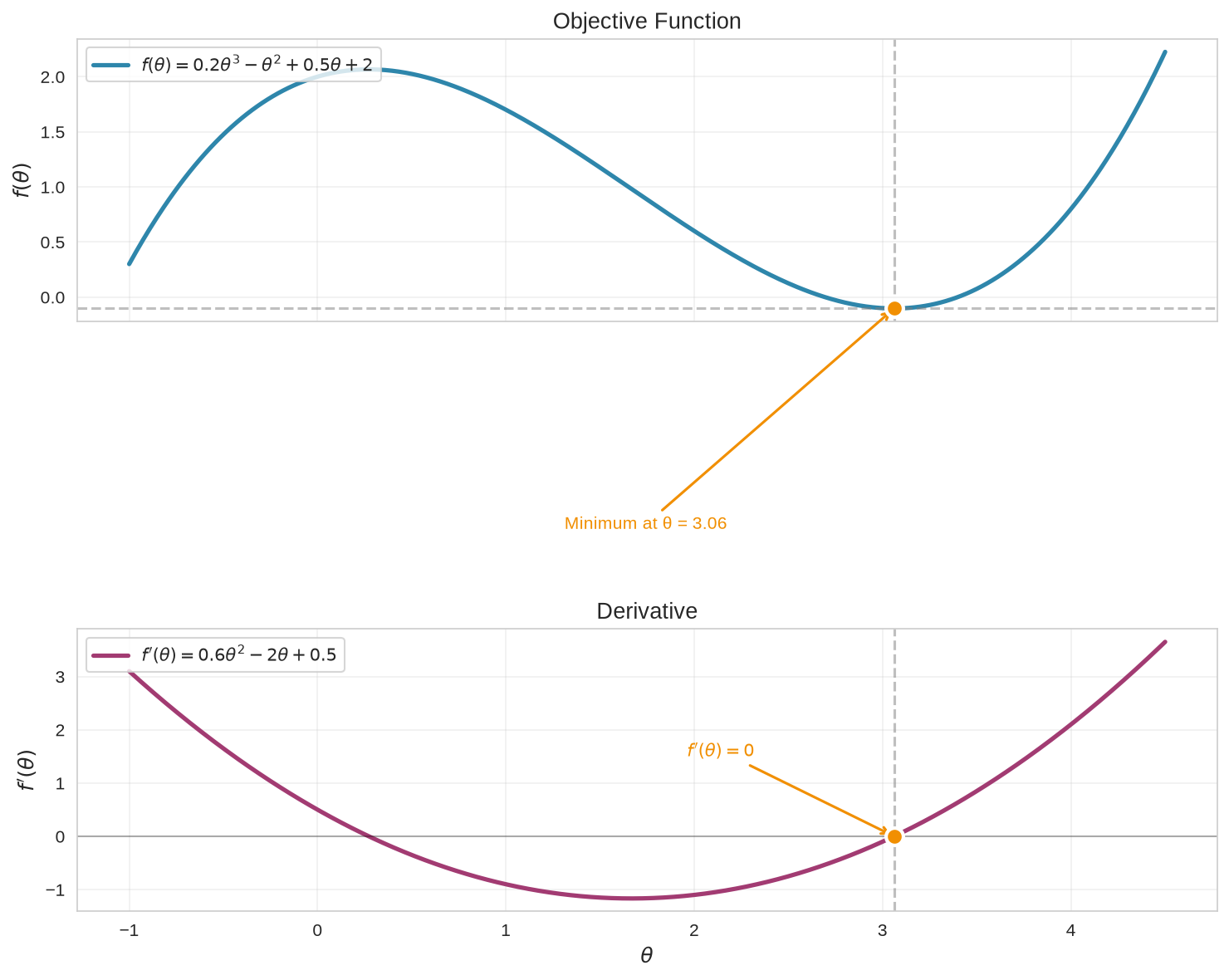
Figure 1:Simple optimization of a univariate function showing the critical point where the derivative equals zero
2.2Gradient Descent Concept
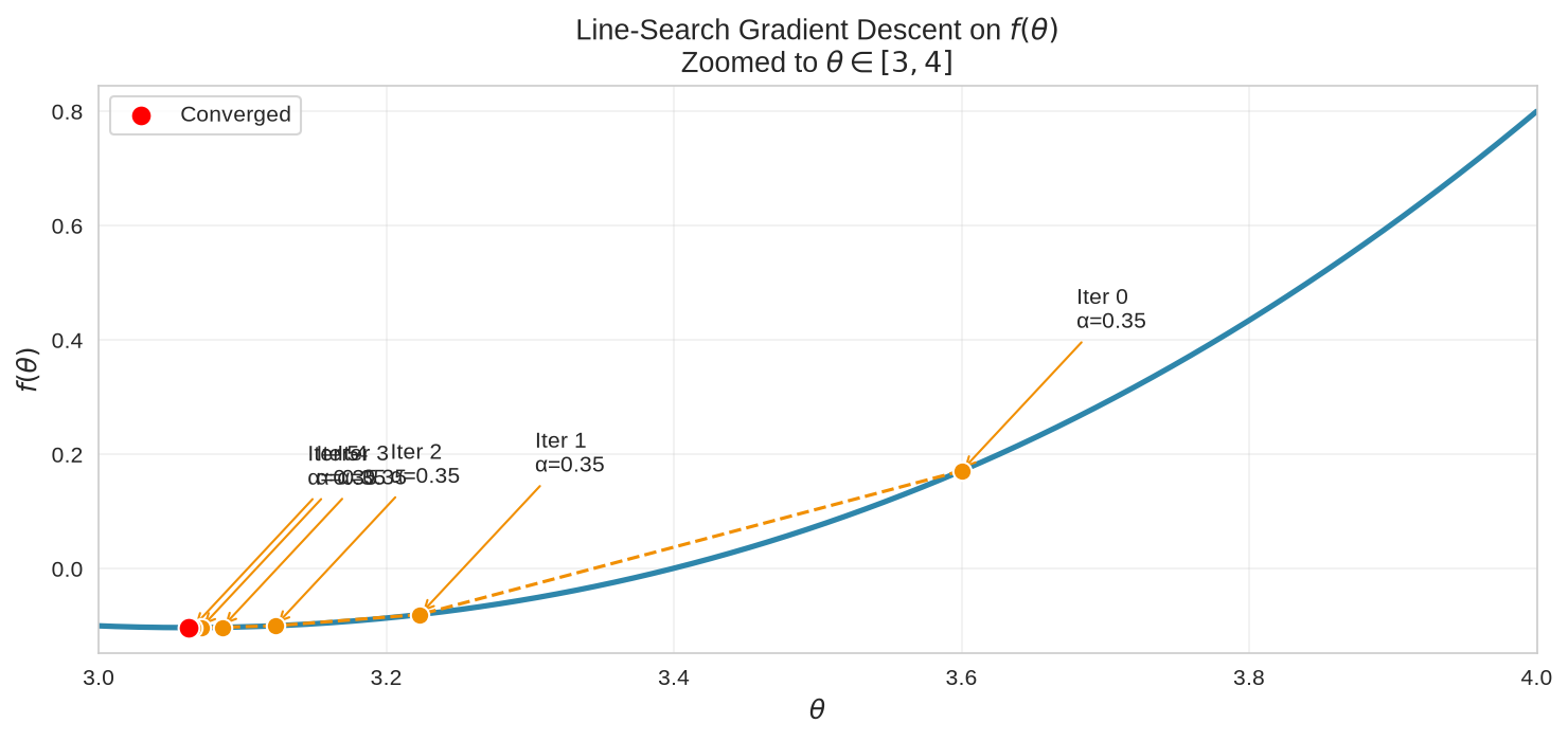
Many FEMU-style objectives are available only through simulations or noisy measurements. Computing symbolically is then impossible, and numerical root-finding can be prohibitively expensive because each trial requires a full model evaluation. Gradient descent offers a practical alternative: repeatedly move in the direction opposite the gradient, reducing the objective without requiring a closed-form solution.
The following visualization applies gradient descent to the objective function. Starting from an arbitrary guess, each step moves downhill along using a line search to select the step length that minimizes along that direction. After a few iterations, the iterates converge to the minimum identified analytically above.
2.3Gradient Descent for Multivariate Functions
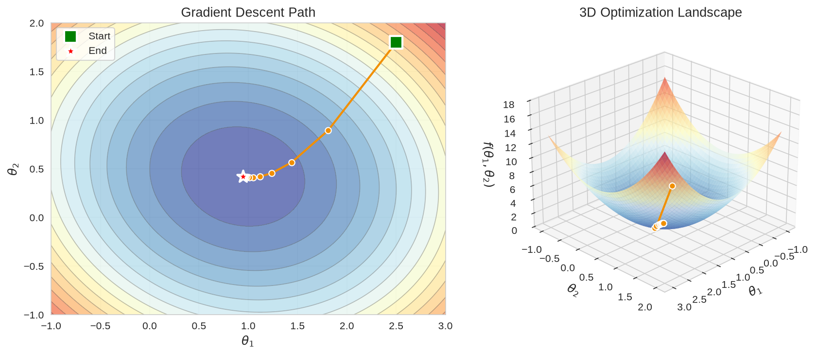
Real engineering problems involve optimizing functions of many variables, such as calibrating a finite element model with many parameters or selecting sensor locations from hundreds of candidates. For a multivariate function where , we extend the derivative to the gradient vector:
The gradient points in the direction of steepest increase. To minimize the function, we move in the opposite direction:
where is the learning rate (step size). Iteration continues until convergence, typically when for some small tolerance .
3Gradient-Free Optimization Methods: Genetic Algorithm
Many optimization problems in structural health monitoring cannot be solved effectively with gradient-based methods. The objective function may be discontinuous, non-differentiable, or expensive to evaluate. Sensor placement involves discrete decisions that create a combinatorial search space, and damage detection objectives often have multiple local minima. These challenges motivate gradient-free methods that explore the solution space without requiring derivative information.
Genetic algorithms mimic biological evolution. The algorithm maintains a population of candidate solutions that evolve through selection, crossover, and mutation. Better solutions are more likely to pass their characteristics to the next generation, gradually improving overall population fitness. This population-based approach maintains diversity and explores multiple regions of the search space simultaneously, reducing sensitivity to local minima.
1 2 3 4 5 6 7 8 9 10 11 12 13from scipy.optimize import differential_evolution def multimodal_function(theta): return theta[0] * np.sin(4*np.pi*theta[0]) - theta[1] * np.sin(4*np.pi*theta[1] + np.pi) + 1 result_ga = differential_evolution( multimodal_function, bounds=[(-1, 1), (-1, 1)], seed=42, maxiter=100, popsize=15 ) print("Best θ:", result_ga.x, "Objective:", result_ga.fun)
Source
from scipy.optimize import differential_evolution
import numpy as np
import matplotlib.pyplot as plt
import pandas as pd

def multimodal_function(theta):
    return theta[0] * np.sin(4*np.pi*theta[0]) - theta[1] * np.sin(4*np.pi*theta[1] + np.pi) + 1

bounds = [(-1, 1), (-1, 1)]

result_ga = differential_evolution(
    multimodal_function,
        bounds,
        seed=42,
    maxiter=100,
    popsize=15,
    polish=True
)

# Visualization
theta_range = np.linspace(-1, 1, 200)
THETA1, THETA2 = np.meshgrid(theta_range, theta_range)
Z = np.zeros_like(THETA1)
for i in range(THETA1.shape[0]):
    for j in range(THETA1.shape[1]):
        Z[i, j] = multimodal_function([THETA1[i, j], THETA2[i, j]])

fig = plt.figure(figsize=(12, 5))

# Contour plot
ax1 = fig.add_subplot(1, 2, 1)
ax1.contour(THETA1, THETA2, Z, levels=20, colors='gray', alpha=0.3, linewidths=0.5)
ax1.contourf(THETA1, THETA2, Z, levels=20, cmap='RdYlBu_r', alpha=0.6)
ax1.scatter(result_ga.x[0], result_ga.x[1], s=200, color='#F18F01',
           marker='*', edgecolor='white', linewidth=2, zorder=5)
ax1.set_xlabel('$\\theta_1$')
ax1.set_ylabel('$\\theta_2$')
ax1.set_title(f'Genetic Algorithm Optimum\nf* = {result_ga.fun:.4f}')
ax1.grid(True, alpha=0.3)

# Surface plot
ax2 = fig.add_subplot(1, 2, 2, projection='3d')
ax2.plot_surface(THETA1, THETA2, Z, cmap='RdYlBu_r', alpha=0.8, edgecolor='none')
ax2.scatter(result_ga.x[0], result_ga.x[1], result_ga.fun,
            s=200, color='#F18F01', marker='*', edgecolor='white', linewidth=1.5)
ax2.set_xlabel('$\\theta_1$')
ax2.set_ylabel('$\\theta_2$')
ax2.set_zlabel('$f(\\theta)$')
ax2.set_title('Surface View of Objective')

plt.tight_layout()
plt.show()

ga_summary = pd.DataFrame({
    'Method': ['Genetic Algorithm'],
    'Optimal θ₁': [f'{result_ga.x[0]:.4f}'],
    'Optimal θ₂': [f'{result_ga.x[1]:.4f}'],
    'Objective Value': [f'{result_ga.fun:.4f}'],
    'Function Evaluations': [result_ga.nfev]
})

display(ga_summary.style.set_caption("Genetic Algorithm Result").hide(axis='index').set_properties(**{'text-align': 'left'}))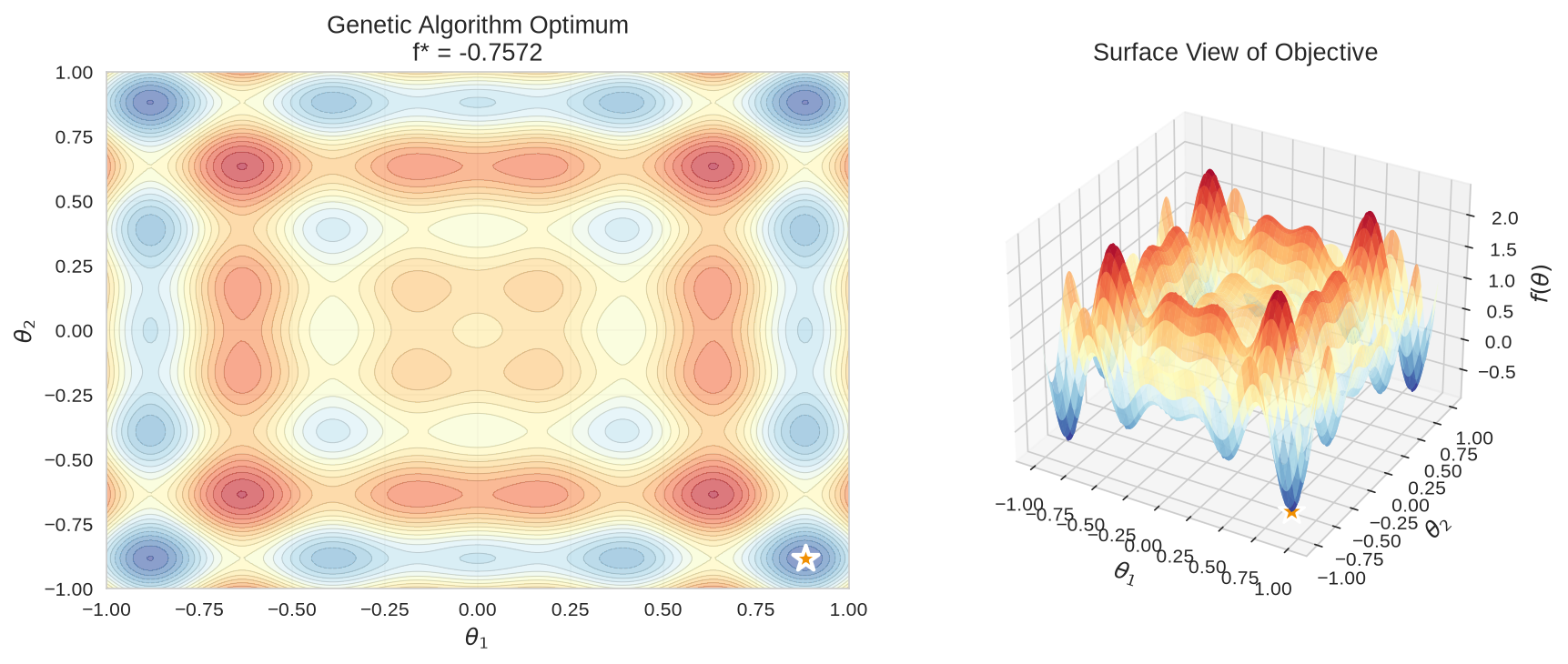
Figure 3:Genetic algorithm locating the global optimum of a multimodal function (line numbers highlight the evolutionary loop)
4Application 1: Finite Element Model Updating and Damage Localization
4.1The Inverse Problem in Structural Identification
Finite element model updating (FEMU) addresses an inverse problem: given measured structural responses, determine the physical parameters that produce those responses. This contrasts with forward analysis, where responses are computed from known parameters. In damage detection, FEMU identifies localized stiffness reductions by calibrating model parameters to match measured modal properties.
FEMU treats damage identification as an optimization problem. We parameterize unknown stiffness modifications, then search for parameter values that minimize discrepancies between model predictions and measurements. Unlike data-driven methods, FEMU uses physics-based models to produce interpretable damage indicators directly linked to structural mechanics.
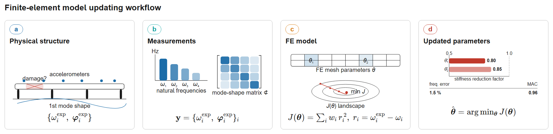
Figure 4:Finite-element model-updating workflow for damage identification. The iterative process adjusts FE model parameters to minimize the residual between predicted and measured modal properties .
4.2Problem Formulation
Consider a two-span continuous bridge with span lengths m and m. Structural stiffness depends on the moment of inertia through the flexural rigidity . Damage reduces local stiffness, modeled here as a multiplicative factor on each span’s moment of inertia.
The damage parameter vector contains the stiffness retention factor for each span, with . A healthy span has ; indicates 30% stiffness loss. The effective moment of inertia is:
where is the baseline moment of inertia.
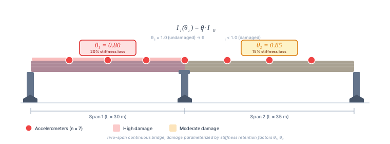
Figure 5:Two-span continuous bridge with damage parameterization. Stiffness retention factors and quantify structural integrity in each span, where indicates no damage and represents stiffness reduction. Accelerometers (red circles) measure modal responses at selected locations.
The complete code for generating modal measurements is shown below:
Modal Analysis in OpenSeeS Utility
1 2 3 4 5 6 7 8 9 10 11 12 13 14 15 16 17 18 19 20 21 22 23 24 25 26 27 28 29 30 31 32 33 34 35 36 37 38 39 40 41 42 43 44 45 46 47 48 49 50 51 52 53 54 55 56 57 58 59 60 61 62 63 64 65 66 67 68 69 70 71 72 73 74 75 76 77 78 79 80 81 82 83 84 85 86 87 88 89 90 91 92 93 94 95 96 97 98 99 100 101 102 103 104 105 106 107 108 109 110 111 112 113 114 115 116 117 118 119 120 121 122 123 124 125 126 127 128 129 130 131 132 133 134 135 136 137 138 139 140""" Modal Measurement Script for FEMU Generates synthetic measured modal data from a damaged structure. Note: This script expects modal_analysis_utility to be in sys.path. """ import numpy as np import matplotlib.pyplot as plt from scipy.interpolate import CubicSpline import os def generate_modal_measurements(save_figures=False): from modal_analysis_utility import ModalAnalysis """ Generate synthetic measured modal data from damaged structure. Parameters: ----------- save_figures : bool If True, save mode shape plots to ch08_figures/ Returns: -------- dict : Dictionary containing all measurement data """ np.random.seed(42) # True damage scenario: 30% damage in span 1, 20% in span 2 theta_true = np.array([0.70, 0.80]) # Create "measured" data from damaged structure spans = [30, 80] supports = ['hinge', 'roller', 'roller'] E, rho, A, I_base = 25e9, 2500, 8.0, 2.67 modal_true = ModalAnalysis(spans, supports, E=E, rho=rho, A=A, I=I_base, I_factors=theta_true) # Run analysis to get results result_true = modal_true.analyze(n_modes=4, plot=False) # Add measurement noise noise_freq = 0.01 noise_mode = 0.02 freq_meas = result_true['frequencies'] * (1 + noise_freq * np.random.randn(4)) modes_meas = result_true['mode_shapes'] + noise_mode * np.random.randn(*result_true['mode_shapes'].shape) # Normalize measured mode shapes for i in range(modes_meas.shape[1]): modes_meas[:, i] /= np.max(np.abs(modes_meas[:, i])) # Create and save mode shape figure if requested if save_figures: script_dir = os.path.dirname(os.path.abspath(__file__)) fig_dir = os.path.join(script_dir, '..', 'ch08_figures') os.makedirs(fig_dir, exist_ok=True) # Create the plot manually (replicate _plot_mode_shapes logic) n_modes = 4 n_cols = 2 n_rows = 2 fig, axes = plt.subplots(n_rows, n_cols, figsize=(14, 10)) for mode_idx in range(n_modes): row = mode_idx // n_cols col = mode_idx % n_cols ax = axes[row, col] mode_num = mode_idx + 1 mode_shape = result_true['mode_shapes'][:, mode_idx] node_positions = result_true['node_positions'] # Enforce zero at supports plot_x = node_positions.copy() plot_y = mode_shape.copy() support_positions = [0, spans[0], spans[0] + spans[1]] for support_x in support_positions: support_idx = np.argmin(np.abs(node_positions - support_x)) plot_y[support_idx] = 0.0 # Smooth curve with spline unique_x, unique_indices = np.unique(plot_x, return_index=True) unique_y = plot_y[unique_indices] if len(unique_x) > 3: spline = CubicSpline(unique_x, unique_y) x_smooth = np.linspace(unique_x.min(), unique_x.max(), 500) y_smooth = spline(x_smooth) ax.plot(x_smooth, y_smooth, 'b-', linewidth=2, label='Mode Shape') else: ax.plot(unique_x, unique_y, 'b-', linewidth=2, label='Mode Shape') # Add support triangles for support_x in support_positions: triangle_height = 0.2 triangle = plt.Polygon([ [support_x - 1.5, -triangle_height], [support_x + 1.5, -triangle_height], [support_x, 0] ], color='green', alpha=0.6, zorder=5) ax.add_patch(triangle) # Add frequency and period text freq = result_true['frequencies'][mode_idx] period = result_true['periods'][mode_idx] ax.text(0.02, 0.98, f'f = {freq:.3f} Hz\nT = {period:.3f} s', transform=ax.transAxes, fontsize=10, verticalalignment='top', bbox=dict(boxstyle='round', facecolor='wheat', alpha=0.5)) # Formatting total_length = sum(spans) ax.set_xlim(-2, total_length + 2) ax.set_ylim(-1.05, 1.05) ax.axhline(y=0, color='k', linestyle='--', linewidth=0.5, alpha=0.3) ax.set_xlabel('Position (m)', fontsize=11) ax.set_ylabel('Amplitude', fontsize=11) ax.set_title(f'Mode {mode_num}', fontsize=12, fontweight='bold') ax.grid(True, alpha=0.3) plt.tight_layout() # Save the figure fig.savefig(os.path.join(fig_dir, 'modal_measurements.png'), dpi=150, bbox_inches='tight') plt.close(fig) return { 'theta_true': theta_true, 'spans': spans, 'supports': supports, 'E': E, 'rho': rho, 'A': A, 'I_base': I_base, 'result_true': result_true, 'freq_meas': freq_meas, 'modes_meas': modes_meas }
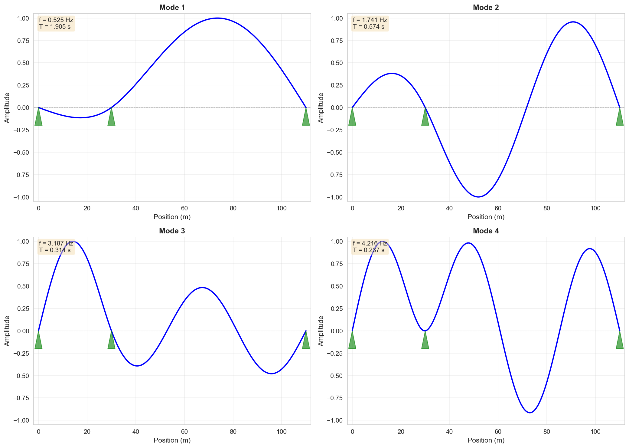
Figure 6:Mode shapes and natural frequencies of the damaged bridge structure. The plot shows the first four vibration modes with their corresponding frequencies and periods.
The forward model performs eigenvalue analysis on the damaged structure, yielding natural frequencies and mode shapes at sensor locations. The inverse problem minimizes the discrepancy between predicted and measured modal properties:
where is the number of measured modes, and are weighting factors, and is the Modal Assurance Criterion for mode :
The MAC quantifies mode shape correlation, ranging from 0 (orthogonal) to 1 (identical). The dual objective uses both frequency and spatial information to guide identification.
4.3Gradient-Based Model Updating
Gradient-based optimization uses derivative information to navigate parameter space. For FEMU, we compute the gradient using automatic differentiation, avoiding finite difference approximations. The update rule is:
where is the step size from a line search. We constrain to ensure physically reasonable stiffness values.
The following implementation uses PyTorch for automatic differentiation. The complete code is shown below:
Gradient-based FEMU implementation script
1 2 3 4 5 6 7 8 9 10 11 12 13 14 15 16 17 18 19 20 21 22 23 24 25 26 27 28 29 30 31 32 33 34 35 36 37 38 39 40 41 42 43 44 45 46 47 48 49 50 51 52 53 54 55 56 57 58 59 60 61 62 63 64 65 66 67 68 69 70 71 72 73 74 75 76 77 78 79 80 81 82 83 84 85 86 87 88 89 90 91 92 93 94 95 96 97 98 99 100 101 102 103 104 105 106 107 108 109 110 111 112 113 114 115 116 117 118 119 120 121 122 123 124 125 126 127 128 129 130 131 132 133 134 135 136 137 138 139 140 141 142 143 144""" Gradient-Based FEMU Script Performs gradient descent optimization for finite element model updating. Generates and saves all visualization figures. Note: This script expects modal_analysis_utility to be in sys.path and measurement data variables to be available in the calling scope. """ import numpy as np import torch import torch.nn as nn import torch.optim as optim import matplotlib.pyplot as plt import seaborn as sns import os import json def run_gradient_femu(theta_true, spans, supports, E, rho, A, I_base, freq_meas, modes_meas, result_true): """ Run gradient-based FEMU and generate all figures. Parameters: ----------- theta_true : array True damage parameters spans : list Span lengths supports : list Support types E, rho, A, I_base : float Material and geometric properties freq_meas : array Measured frequencies modes_meas : array Measured mode shapes result_true : dict True modal analysis results """ from modal_analysis_utility import ModalAnalysis sns.set_style('whitegrid') plt.rcParams.update({'font.size': 10, 'figure.dpi': 100}) torch.manual_seed(42) # Define helper functions inside the main function to access parameters def run_modal_analysis(theta_values): """Utility wrapper to ensure consistent calls to ModalAnalysis.""" theta_values = np.clip(np.array(theta_values, dtype=float), 0.5, 1.0) modal = ModalAnalysis(spans, supports, E=E, rho=rho, A=A, I=I_base, I_factors=theta_values) return modal.analyze(n_modes=4, plot=False) class ModalAnalysisAutograd(torch.autograd.Function): """Custom autograd function with finite-difference gradients.""" eps = 1e-3 @staticmethod def forward(ctx, theta_tensor): theta_numpy = theta_tensor.detach().cpu().numpy() result = run_modal_analysis(theta_numpy) ctx.save_for_backward(theta_tensor.detach().clone()) return (torch.tensor(result['frequencies'], dtype=torch.float32, device=theta_tensor.device), torch.tensor(result['mode_shapes'], dtype=torch.float32, device=theta_tensor.device)) @staticmethod def backward(ctx, grad_freq, grad_modes): (theta_saved,) = ctx.saved_tensors eps = ModalAnalysisAutograd.eps if grad_freq is None: grad_freq = torch.zeros(4, device=theta_saved.device) if grad_modes is None: grad_modes = torch.zeros(result_true['mode_shapes'].shape, device=theta_saved.device) grad_theta = torch.zeros_like(theta_saved) for i in range(len(theta_saved)): theta_plus = theta_saved.clone() theta_minus = theta_saved.clone() theta_plus[i] = torch.clamp(theta_plus[i] + eps, 0.5, 1.0) theta_minus[i] = torch.clamp(theta_minus[i] - eps, 0.5, 1.0) res_plus = run_modal_analysis(theta_plus.cpu().numpy()) res_minus = run_modal_analysis(theta_minus.cpu().numpy()) freq_plus = torch.tensor(res_plus['frequencies'], dtype=torch.float32, device=grad_freq.device) freq_minus = torch.tensor(res_minus['frequencies'], dtype=torch.float32, device=grad_freq.device) modes_plus = torch.tensor(res_plus['mode_shapes'], dtype=torch.float32, device=grad_modes.device) modes_minus = torch.tensor(res_minus['mode_shapes'], dtype=torch.float32, device=grad_modes.device) freq_grad = (freq_plus - freq_minus) / (2 * eps) modes_grad = (modes_plus - modes_minus) / (2 * eps) grad_theta[i] = torch.sum(grad_freq * freq_grad) + torch.sum(grad_modes * modes_grad) return (grad_theta.to(theta_saved.device),) class FEMUModel(nn.Module): """FEMU model with gradient computation""" def __init__(self, initial_theta=[0.95, 0.95]): super().__init__() self.psi = nn.Parameter(torch.tensor(initial_theta, dtype=torch.float32)) def get_theta(self): """Convert unconstrained ψ to constrained θ ∈ [0.5, 1.0]""" return 0.5 + 0.5 * torch.sigmoid(self.psi) def forward(self, freq_target, modes_target, w_freq=1.0, w_mac=0.5): """Compute objective function""" theta_current = self.get_theta() freq_pred, modes_pred = ModalAnalysisAutograd.apply(theta_current) freq_error = torch.sum(((freq_pred - freq_target) / freq_target)**2) mac_sum = 0.0 for i in range(4): mode_pred = modes_pred[:, i] mode_meas = modes_target[:, i] numerator = torch.abs(torch.dot(mode_pred, mode_meas))**2 denominator = torch.dot(mode_pred, mode_pred) * torch.dot(mode_meas, mode_meas) mac = numerator / (denominator + 1e-8) mac_sum += (1 - mac) J = w_freq * freq_error + w_mac * mac_sum return J, freq_pred, modes_pred # Gradient-based optimization model = FEMUModel(initial_theta=[0.95, 0.95]) optimizer = optim.Adam(model.parameters(), lr=0.05) freq_target = torch.tensor(freq_meas, dtype=torch.float32) modes_target = torch.tensor(modes_meas, dtype=torch.float32) history_grad = {'iteration': [], 'objective': [], 'theta_1': [], 'theta_2': [], 'freq': [], 'modes': []} n_iterations = 200 for iteration in range(n_iterations): optimizer.zero_grad() J, freq_pred, modes_pred = model(freq_target, modes_target, w_freq=1.0, w_mac=0.5) J.backward() optimizer.step() theta_current = model.get_theta().detach().numpy() if iteration % 10 == 0: history_grad['iteration'].append(iteration) history_grad['objective'].append(J.item()) history_grad['theta_1'].append(theta_current[0]) history_grad['theta_2'].append(theta_current[1]) history_grad['freq'].append(freq_pred.detach().numpy().copy()) history_grad['modes'].append(modes_pred.detach().numpy().copy()) theta_grad_final = model.get_theta().detach().numpy()
Skipping gradient FEMU execution (CI environment or OpenSees not available)
Results will be loaded from pre-generated figures
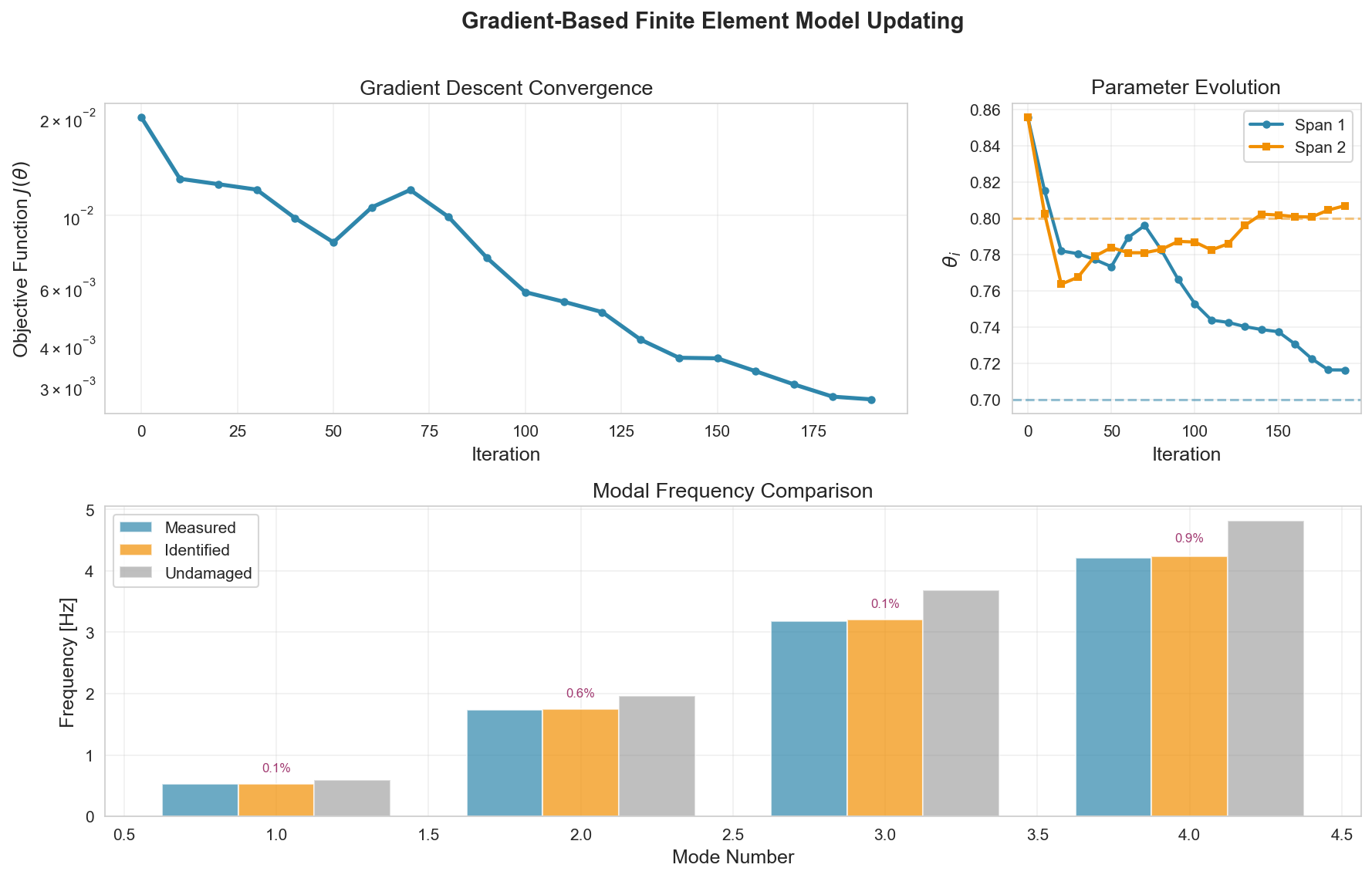
Figure 7:Gradient-based FEMU optimization results showing convergence history, parameter evolution, and modal frequency comparison between measured, identified, and undamaged states.
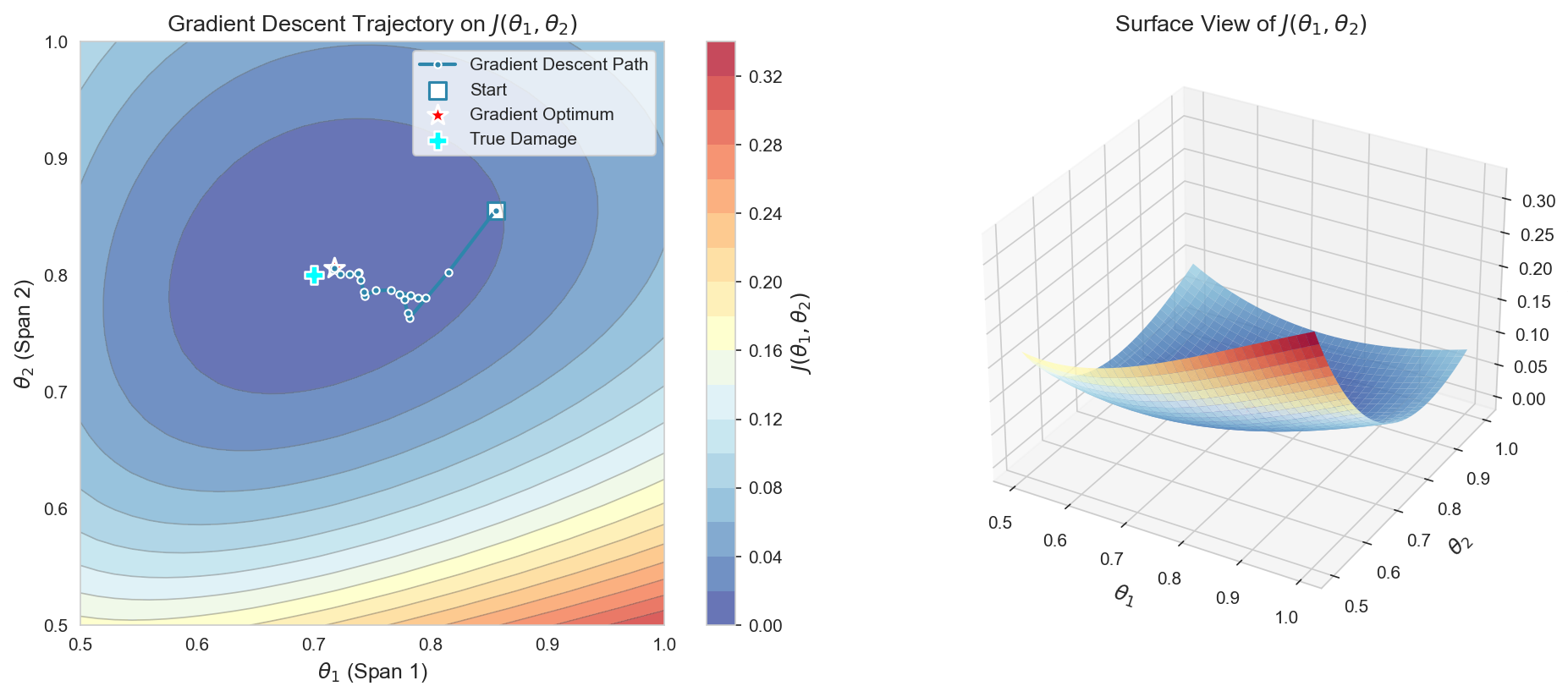
Figure 8:Optimization landscape showing the objective function with gradient descent trajectory from initial guess to optimum, displayed in both 2D contour and 3D surface views.
4.4Genetic Algorithm for Model Updating
Gradient-free methods are useful when objective functions are non-smooth or derivatives are unavailable. Genetic algorithms (GA) maintain a population of candidate solutions and evolve them through selection, crossover, and mutation. This population-based search explores multiple regions simultaneously, reducing sensitivity to local minima.
For FEMU, each individual encodes a damage hypothesis . The fitness equals , since GAs maximize fitness. Selection favors individuals with lower , crossover combines parent solutions, and mutation maintains exploration.
The implementation uses scipy.optimize.differential_evolution, a GA variant with strong convergence properties. The complete code is shown below:
Genetic Algorithm FEMU implementation script
1 2 3 4 5 6 7 8 9 10 11 12 13 14 15 16 17 18 19 20 21 22 23 24 25 26 27 28 29 30 31 32 33 34 35 36 37 38 39 40 41 42 43 44 45 46 47 48 49 50 51 52 53 54 55 56 57 58 59 60 61 62 63 64 65 66 67 68 69 70 71 72 73 74 75 76 77 78 79 80 81 82 83 84 85 86 87 88 89 90 91 92 93 94 95 96 97 98 99 100 101 102 103 104 105 106 107 108 109 110 111 112 113 114 115 116 117 118""" Genetic Algorithm FEMU Script Performs GA optimization for finite element model updating. Generates and saves all visualization figures. Note: This script expects modal_analysis_utility to be in sys.path and measurement data variables to be available in the calling scope. """ import numpy as np import matplotlib.pyplot as plt import seaborn as sns from scipy.optimize import differential_evolution import time import os import json def run_ga_femu(theta_true, spans, supports, E, rho, A, I_base, freq_meas, modes_meas, result_true): """ Run GA-based FEMU and generate all figures. Parameters: ----------- theta_true : array True damage parameters spans : list Span lengths supports : list Support types E, rho, A, I_base : float Material and geometric properties freq_meas : array Measured frequencies modes_meas : array Measured mode shapes result_true : dict True modal analysis results """ from modal_analysis_utility import ModalAnalysis sns.set_style('whitegrid') plt.rcParams.update({'font.size': 10, 'figure.dpi': 100}) # Define objective function inside to access parameters def objective_function_ga(theta_vec): """Objective function for GA optimization""" modal = ModalAnalysis(spans, supports, E=E, rho=rho, A=A, I=I_base, I_factors=theta_vec) result = modal.analyze(n_modes=4, plot=False) freq_pred = result['frequencies'] modes_pred = result['mode_shapes'] freq_error = np.sum(((freq_pred - freq_meas) / freq_meas)**2) mac_error = 0.0 for i in range(4): mode_p = modes_pred[:, i] mode_m = modes_meas[:, i] numerator = np.abs(np.dot(mode_p, mode_m))**2 denominator = np.dot(mode_p, mode_p) * np.dot(mode_m, mode_m) mac = numerator / (denominator + 1e-10) mac_error += (1 - mac) J = 1.0 * freq_error + 0.5 * mac_error return J bounds = [(0.5, 1.0), (0.5, 1.0)] popsize = 15 history_ga = {'generation': [], 'objective': [], 'theta_1': [], 'theta_2': []} ga_iter_counter = {'value': 0} def callback_ga(xk, convergence): """Callback to record optimization history""" iter_idx = ga_iter_counter['value'] history_ga['generation'].append(iter_idx) history_ga['objective'].append(objective_function_ga(xk)) history_ga['theta_1'].append(float(xk[0])) history_ga['theta_2'].append(float(xk[1])) ga_iter_counter['value'] += 1 return False # Initialize population near [0.95, 0.95] np.random.seed(42) dim = len(bounds) init_base = np.array([0.95, 0.95]) init_pop = np.tile(init_base, (popsize * dim, 1)) init_pop += 0.02 * np.random.uniform(-1, 1, size=init_pop.shape) lower_bounds = np.array([b[0] for b in bounds]) upper_bounds = np.array([b[1] for b in bounds]) init_pop = np.clip(init_pop, lower_bounds, upper_bounds) start_time = time.time() result_ga = differential_evolution( objective_function_ga, bounds, strategy='best1bin', maxiter=100, popsize=popsize, mutation=(0.5, 1.0), recombination=0.7, seed=42, callback=callback_ga, polish=True, workers=1, init=init_pop ) ga_time = time.time() - start_time theta_ga_final = result_ga.x # Ensure final optimum is recorded history_ga['generation'].append(ga_iter_counter['value']) history_ga['objective'].append(result_ga.fun) history_ga['theta_1'].append(float(theta_ga_final[0])) history_ga['theta_2'].append(float(theta_ga_final[1])) modal_ga_final = ModalAnalysis(spans, supports, E=E, rho=rho, A=A, I=I_base, I_factors=theta_ga_final) result_ga_final = modal_ga_final.analyze(n_modes=4, plot=False)
Skipping GA FEMU execution (CI environment or OpenSees not available)
Results will be loaded from pre-generated figures
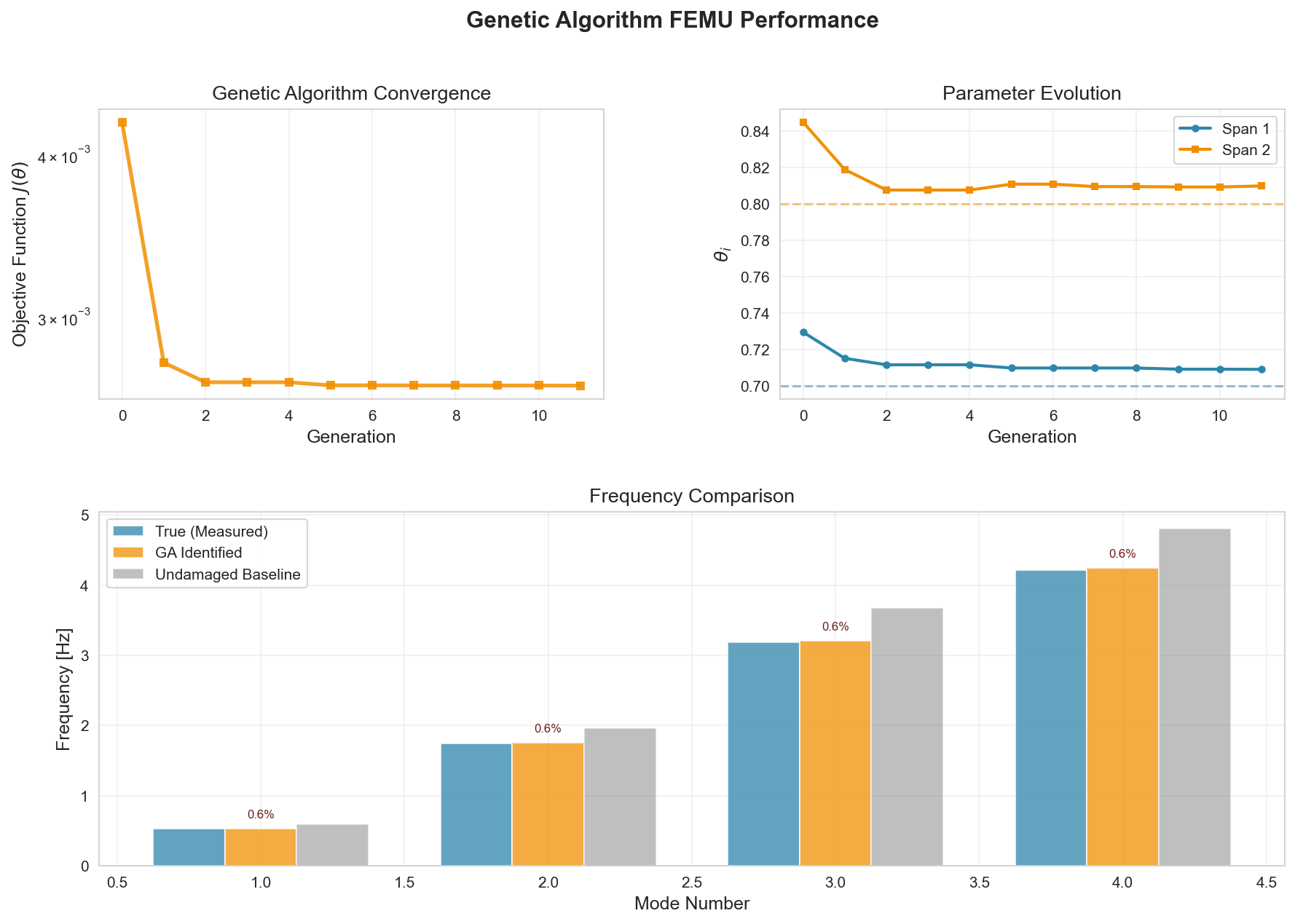
Figure 9:Genetic Algorithm FEMU optimization results showing convergence history across generations, parameter evolution for both spans, and modal frequency comparison between measured, GA-identified, and undamaged states.
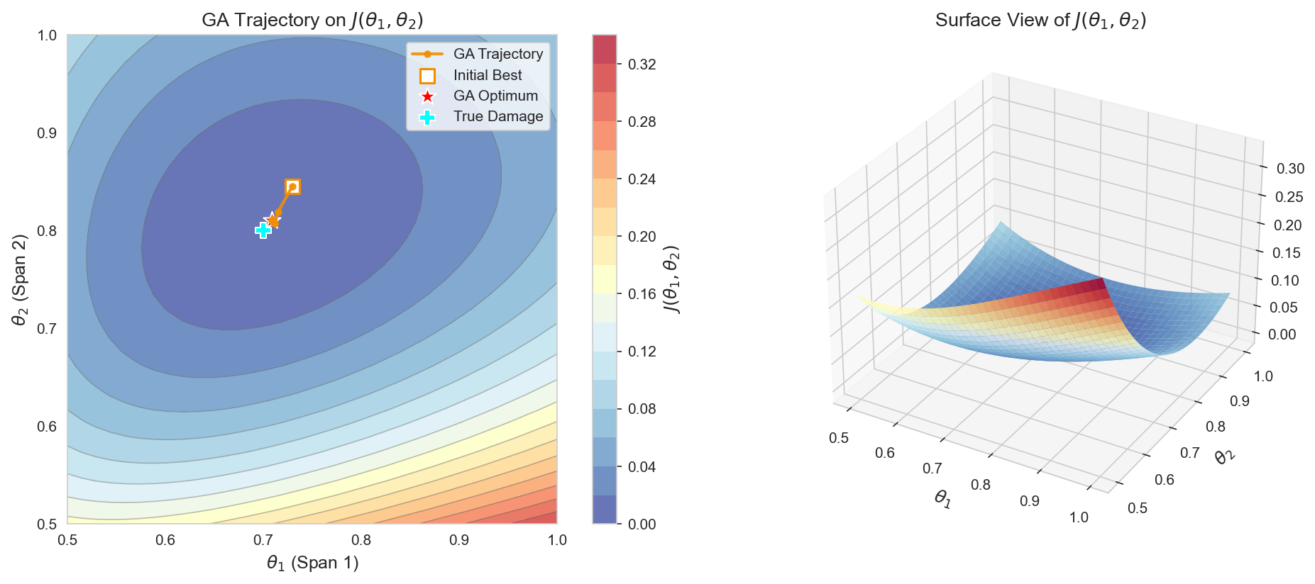
Figure 10:Optimization landscape showing the objective function with Genetic Algorithm trajectory from initial population to final optimum, displayed in both 2D contour and 3D surface views.
5Application 2: Optimal Sensor Placement
Sensor placement decisions directly affect monitoring system effectiveness. With a limited sensor budget, the goal is to maximize information content while minimizing redundancy, so that modal parameters can be accurately identified from the measured responses.
5.1Information-Based Placement Criterion
We select sensors from candidate locations by maximizing the Fisher Information Matrix (FIM). For modal analysis, the FIM quantifies mode shape observability:
where contains mode shapes at sensor locations. The D-optimality criterion maximizes the determinant:
Large determinant values indicate well-conditioned mode shape matrices where modes remain distinguishable despite measurement noise, preventing ill-conditioning during modal parameter extraction.
5.2Genetic Algorithm Implementation
Sensor placement is a combinatorial problem: selecting from locations yields possible configurations. For a bridge with 50 candidate locations and 8 sensors, this exceeds 500 million configurations. Genetic algorithms search this discrete space through evolutionary operations without exhaustive enumeration.
We use differential evolution, which encodes sensor locations as continuous variables and selects the largest values. This continuous relaxation improves convergence while preserving discrete sensor assignments.
5.3Two-Span Bridge Example
We apply optimal sensor placement to the two-span continuous bridge from the FEMU example (Figure 5), which has spans of 30 m and 80 m for a total length of 110 m. A finite element model with 0.5 m mesh spacing is used to perform modal analysis on the intact structure and extract mode shapes at potential sensor locations.
5.3.1Modal Analysis for Sensor Grid
Candidate sensor locations are defined at 2.5 m intervals starting from 2.5 m, excluding support positions. This yields uniformly distributed accelerometer candidates across the bridge deck. We extract the first four mode shapes at these locations, as they contain the most significant structural information for damage detection.
The following code demonstrates the modal analysis utility used to generate the sensor grid data:
Modal Analysis Utility for Sensor Grid
1 2 3 4 5 6 7 8 9 10 11 12 13 14 15 16 17 18 19 20 21 22 23 24 25 26 27 28 29 30 31 32 33 34 35 36 37 38 39 40 41 42 43 44 45 46 47 48 49 50 51 52 53 54 55 56 57 58 59 60 61 62 63 64 65 66 67 68 69 70 71 72 73 74 75 76 77 78 79 80 81 82 83 84 85 86 87 88 89 90 91 92 93 94 95 96 97 98 99 100 101 102""" Generate modal data for sensor grid locations using FE model. This script performs modal analysis on the intact bridge structure and extracts mode shape amplitudes at candidate sensor locations for optimal sensor placement. """ import numpy as np import matplotlib.pyplot as plt import json import os import sys def generate_sensor_grid_data(save_data=True): """ Generate modal data at sensor grid locations for optimal sensor placement. Parameters ---------- save_data : bool If True, save the sensor grid data to JSON file Returns ------- dict Dictionary containing sensor locations and mode shape data """ # Add path to common utilities script_dir = os.path.dirname(os.path.abspath(__file__)) project_root = os.path.abspath(os.path.join(script_dir, '..', '..', '..')) common_util_path = os.path.join(project_root, 'common_utility_data') if common_util_path not in sys.path: sys.path.insert(0, common_util_path) from modal_analysis_utility import ModalAnalysis # Bridge geometry (same as FEMU example) spans = [30.0, 80.0] # Two-span continuous bridge supports = ['hinge', 'roller', 'roller'] # Support types support_positions = [0.0, 30.0, 110.0] # Support locations # Structural properties E = 30e9 # Young's modulus (Pa) - concrete rho = 2500 # Density (kg/m³) A = 6.0 # Cross-sectional area (m²) I_base = 4.5 # Base moment of inertia (m⁴) # Intact bridge (no damage) I_factors = [1.0, 1.0] # No stiffness reduction # Perform modal analysis on intact structure # Use first 4 modes for sensor placement study modal = ModalAnalysis(spans, supports, E=E, rho=rho, A=A, I=I_base, I_factors=I_factors) result = modal.analyze(n_modes=4, plot=False) # Define sensor grid: every 2.5 m starting from 2.5 m (excluding supports) mesh_size = 0.5 # FE mesh size sensor_spacing = 2.5 # Sensor grid spacing # Generate candidate sensor locations candidate_locations = [] x = 2.5 # Start at 2.5 m while x < 110.0: # Exclude support locations (with 0.1 m tolerance) is_support = any(abs(x - sup) < 0.1 for sup in support_positions) if not is_support: candidate_locations.append(x) x += sensor_spacing candidate_locations = np.array(candidate_locations) n_candidates = len(candidate_locations) # Extract mode shape amplitudes at candidate locations # Interpolate from FE node positions to candidate locations node_positions = modal.node_positions n_modes = 4 mode_shapes_at_candidates = np.zeros((n_candidates, n_modes)) for i, loc in enumerate(candidate_locations): for mode_idx in range(n_modes): # Linear interpolation mode_shape_at_loc = np.interp(loc, node_positions, modal.mode_shapes[:, mode_idx]) mode_shapes_at_candidates[i, mode_idx] = mode_shape_at_loc # Extract frequencies frequencies = modal.frequencies[:n_modes] # Prepare data for saving data = { 'candidate_locations': candidate_locations.tolist(), 'mode_shapes': mode_shapes_at_candidates.tolist(), # sampled at candidate locations 'frequencies': frequencies.tolist(), 'n_modes': n_modes, 'n_candidates': n_candidates, 'bridge_geometry': { 'spans': spans, 'supports': supports, 'support_positions': support_positions, 'total_length': sum(spans) } }
Running in CI environment - using pre-generated sensor grid data.
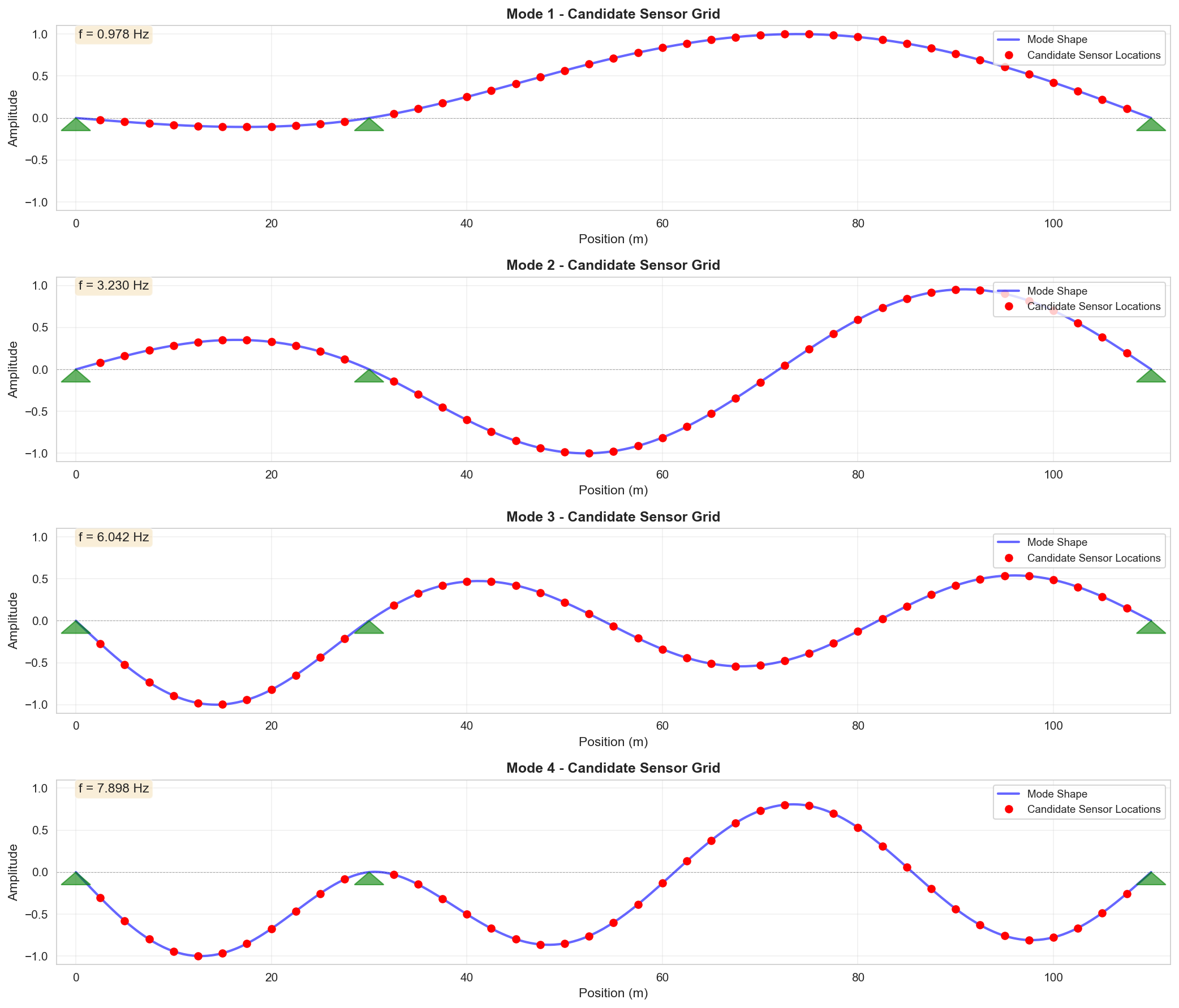
Figure 11:Mode shapes at candidate sensor grid locations.
5.3.2Optimal Sensor Placement Optimization
With modal data available, we determine the optimal placement of 8 accelerometers to maximize observability of the first three modes. The genetic algorithm maximizes the determinant of the Fisher Information Matrix, which measures the information content of a given sensor configuration.
import numpy as np
from scipy.optimize import differential_evolution
from scipy.linalg import svd
import matplotlib.pyplot as plt
import json
import time

with open(data_path, 'r') as f:
    sensor_data = json.load(f)

candidate_locations = np.array(sensor_data['candidate_locations'])
mode_shapes = np.array(sensor_data['mode_shapes'])
frequencies = np.array(sensor_data['frequencies'])
n_sensors = 8

n_candidates = len(candidate_locations)
n_modes = mode_shapes.shape[1]

# Optimization history storage
history = {
    'iteration': [],
    'best_objective': [],
    'best_sensors': []
}
iteration_counter = [0]

def objective_function(x):
    """
    Objective: Maximize determinant of Fisher Information Matrix (FIM).
    We minimize negative log-determinant for numerical stability.
    """
    # Convert continuous variables to discrete sensor selection
    sensor_indices = np.argsort(x)[-n_sensors:]
    sensor_indices = np.sort(sensor_indices)

    # Extract mode shapes at selected sensor locations
    Phi_s = mode_shapes[sensor_indices, :]

    # Fisher Information Matrix: Phi^T * Phi
    FIM = Phi_s.T @ Phi_s

    # Compute log-determinant using SVD for numerical stability
    try:
        _, singular_values, _ = svd(FIM)
        log_det = np.sum(np.log(singular_values + 1e-12))
        return -log_det  # Minimize negative = maximize positive
    except:
        return 1e10  # Penalty for singular matrix

def callback(xk, convergence):
    """Store optimization progress"""
    iteration_counter[0] += 1
    sensor_indices = np.argsort(xk)[-n_sensors:]
    obj_val = objective_function(xk)

    history['iteration'].append(iteration_counter[0])
    history['best_objective'].append(-obj_val)  # Store positive log-det
    history['best_sensors'].append(np.sort(sensor_indices).tolist())

    if iteration_counter[0] % 10 == 0:
        print(f"  Iteration {iteration_counter[0]}: log-det(FIM) = {-obj_val:.4f}")

# Run Genetic Algorithm
print("\nRunning genetic algorithm optimization...")
start_time = time.time()

bounds = [(0, 1) for _ in range(n_candidates)]

result = differential_evolution(
    objective_function,
    bounds,
    strategy='best1bin',
    maxiter=100,
    popsize=20,
    mutation=(0.5, 1.5),
    recombination=0.7,
    seed=42,
    callback=callback,
    disp=False,
    workers=1
)

runtime = time.time() - start_time

# Extract optimal configuration
optimal_x = result.x
optimal_sensor_indices = np.argsort(optimal_x)[-n_sensors:]
optimal_sensor_indices = np.sort(optimal_sensor_indices)
optimal_sensor_locations = candidate_locations[optimal_sensor_indices]

# Compute final metrics
Phi_optimal = mode_shapes[optimal_sensor_indices, :]
FIM_optimal = Phi_optimal.T @ Phi_optimal

# Store iteration count for summary table
n_iterations = len(history['iteration'])

print(f"\nOptimization completed in {runtime:.2f} seconds")
Running genetic algorithm optimization...
Iteration 10: log-det(FIM) = 5.3663
Iteration 20: log-det(FIM) = 5.3663
Iteration 30: log-det(FIM) = 5.3751
Iteration 40: log-det(FIM) = 5.4168
Iteration 50: log-det(FIM) = 5.4286
Iteration 60: log-det(FIM) = 5.4286
Iteration 70: log-det(FIM) = 5.4286
Iteration 80: log-det(FIM) = 5.4286
Iteration 90: log-det(FIM) = 5.4286
  Iteration 100: log-det(FIM) = 5.4286

Optimization completed in 7.48 seconds
Source
fig1, ax1 = plt.subplots(1, 1, figsize=(12, 4.5))

iterations = np.array(history['iteration'])
objectives = np.array(history['best_objective'])

# Plot convergence with gradient effect
ax1.plot(iterations, objectives, linewidth=2.5,
         marker='o', markersize=5, markevery=10,
         markerfacecolor='white', markeredgewidth=2,
         markeredgecolor='#2563eb', color='#2563eb', zorder=3)

# Add shaded region to show improvement
ax1.fill_between(iterations, objectives.min(), objectives,
                 alpha=0.15, color='#2563eb', zorder=1)

# Highlight final value
ax1.plot(iterations[-1], objectives[-1], 'o', markersize=10,
         markerfacecolor='#dc2626', markeredgecolor='white', markeredgewidth=2,
         zorder=4, label=f'Final: {objectives[-1]:.4f}')

ax1.set_xlabel('Iteration', fontsize=12, fontweight='bold')
ax1.set_ylabel('log-det(FIM)', fontsize=12, fontweight='bold')
ax1.set_title('Convergence History', fontsize=13, fontweight='bold', pad=15)
ax1.grid(True, alpha=0.25, linestyle='--', linewidth=0.8)
ax1.set_xlim(-2, max(iterations) * 1.03)
ax1.legend(loc='lower right', framealpha=0.95, edgecolor='gray')
ax1.spines['top'].set_visible(False)
ax1.spines['right'].set_visible(False)

plt.tight_layout()
plt.show()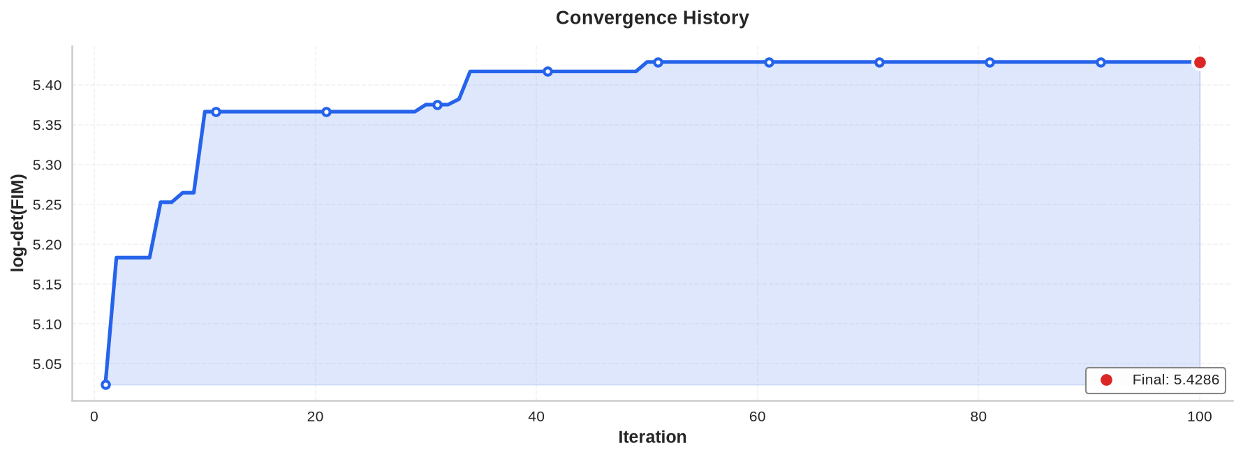
Figure 12:Convergence history showing the log-determinant of the Fisher Information Matrix increasing as the genetic algorithm identifies better sensor configurations.
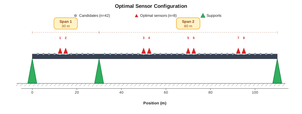
Figure 13:Final optimal configuration with 8 accelerometers (red triangles) distributed across the bridge deck. Gray circles indicate candidate sensor locations, and green triangles represent bridge supports.
Source
fig, axes = plt.subplots(2, 1, figsize=(12, 10))

# Subplot 1: Mode shape coverage with improved styling
ax1 = axes[0]
x_full = np.linspace(0, 110, 500)

# Define color palette for modes
mode_colors = ['#2563eb', '#dc2626', '#16a34a', '#9333ea']

for mode_idx in range(n_modes):
    mode_interp = np.interp(x_full, candidate_locations, mode_shapes[:, mode_idx])
    ax1.plot(x_full, mode_interp, linewidth=2.5, alpha=0.8,
            color=mode_colors[mode_idx], label=f'Mode {mode_idx + 1}')

# Plot sensor locations with improved visibility
for loc in optimal_sensor_locations:
    ax1.axvline(x=loc, color='#dc2626', linestyle='--', linewidth=1.5, alpha=0.4)

# Add zero line
ax1.axhline(y=0, color='gray', linestyle='-', linewidth=0.8, alpha=0.5, zorder=1)

ax1.set_xlabel('Position (m)', fontsize=12, fontweight='bold')
ax1.set_ylabel('Mode Shape Amplitude', fontsize=12, fontweight='bold')
ax1.set_title('Mode Shape Coverage by Optimal Sensors', fontsize=13, fontweight='bold', pad=15)
ax1.legend(loc='upper right', fontsize=10, framealpha=0.95, edgecolor='gray', ncol=2)
ax1.grid(True, alpha=0.25, linestyle='--', linewidth=0.8)
ax1.set_xlim(0, 110)
ax1.spines['top'].set_visible(False)
ax1.spines['right'].set_visible(False)

# Subplot 2: Fisher Information Matrix with improved styling
ax2 = axes[1]

# Use a better colormap for scientific visualization
im = ax2.imshow(FIM_optimal, cmap='RdYlBu_r', aspect='auto',
               interpolation='nearest', vmin=FIM_optimal.min(), vmax=FIM_optimal.max())

ax2.set_xlabel('Mode Index', fontsize=12, fontweight='bold')
ax2.set_ylabel('Mode Index', fontsize=12, fontweight='bold')
ax2.set_title('Fisher Information Matrix', fontsize=13, fontweight='bold', pad=15)
ax2.set_xticks(range(n_modes))
ax2.set_yticks(range(n_modes))
ax2.set_xticklabels([f'{i+1}' for i in range(n_modes)])
ax2.set_yticklabels([f'{i+1}' for i in range(n_modes)])

# Add colorbar with improved styling
cbar = plt.colorbar(im, ax=ax2, fraction=0.046, pad=0.04)
cbar.set_label('FIM Value', fontsize=11, fontweight='bold')
cbar.ax.tick_params(labelsize=10)

# Add text annotations with adaptive color
for i in range(n_modes):
    for j in range(n_modes):
        # Choose text color based on background intensity
        val = FIM_optimal[i, j]
        text_color = 'white' if val > (FIM_optimal.max() * 0.6) else 'black'
        ax2.text(j, i, f'{val:.2f}',
                ha="center", va="center", color=text_color,
                fontsize=10, fontweight='bold')

# Add grid lines between cells
for i in range(n_modes + 1):
    ax2.axhline(i - 0.5, color='white', linewidth=2)
    ax2.axvline(i - 0.5, color='white', linewidth=2)

plt.tight_layout()
plt.show()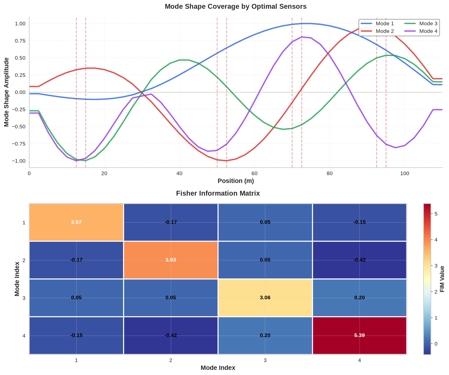
Figure 14:Mode shape observability analysis. Left: Coverage of the first three mode shapes by optimal sensor locations (vertical dashed lines). The sensor distribution captures critical regions where mode shape amplitudes are significant. Right: Fisher Information Matrix showing the information content for each mode pair, with diagonal dominance indicating strong individual mode observability.
Source
import pandas as pd

# Print summary information
print("Optimal Sensor Placement Summary")
print("=" * 50)
print(f"Number of Sensors: {int(n_sensors)}")
print(f"Number of Modes: {int(n_modes)}")
print(f"Candidate Locations: {int(n_candidates)}")
print(f"GA Iterations: {int(n_iterations)}")
print(f"Runtime: {runtime:.2f} s")
print()

# Create sensor locations table
sensor_data = {
    'Sensor #': [f"{i+1}" for i in range(len(optimal_sensor_locations))],
    'Position (m)': [f"{loc:.1f}" for loc in optimal_sensor_locations],
    'Span': ['Span 1' if loc <= 30.0 else 'Span 2' for loc in optimal_sensor_locations]
}

df_sensors = pd.DataFrame(sensor_data)

# Display sensor locations table
display(df_sensors.style.hide(axis='index').set_properties(**{
    'text-align': 'center',
    'font-size': '11pt'
}).set_caption("Optimal Sensor Locations and Properties"))
Optimal Sensor Placement Summary
==================================================
Number of Sensors: 8
Number of Modes: 4
Candidate Locations: 42
GA Iterations: 100
Runtime: 7.48 s
5.3.3Results and Discussion
The genetic algorithm identifies a sensor layout that captures the essential dynamic behavior of the bridge using a limited number of accelerometers. The convergence history shows a steady increase in information content before the solution stabilizes.
The final sensor pattern distributes instruments across both spans, placing sensors near regions of large modal amplitude and away from nodal lines where motion is small. The resulting measurement set is informative for all targeted modes.
In practice, this optimal configuration is a starting point. Actual deployment must account for access, safety, power, cabling, and maintenance. The final layout may require adjustments, but sensors moved short distances from their ideal positions typically retain most of their information content.
5.4Alternative Sensor Placement Approaches
Beyond the Fisher Information approach, other strategies for sensor placement evaluate how well a limited sensor set supports inverse problem solutions. Two practical alternatives use model updating and force identification, respectively.
5.4.1Model Updating Based Placement
This approach treats sensor placement as a model calibration problem. If a small set of sensors provides enough information to accurately identify structural parameters, those sensors are well placed.
The procedure is as follows. Select a trial set of sensor locations from the available candidates. Using only measurements from these sensors, perform system identification to estimate structural parameters (stiffness, mass, or damage indicators). Use the identified model to predict responses at all candidate locations, including those not instrumented. Compare predictions against reference values: low prediction error indicates the trial sensors captured sufficient structural information.
Repeating this process for different trial configurations identifies which sensor combinations yield the lowest prediction errors. The configuration that best reconstructs the full structural response from a subset of measurements is selected as optimal.
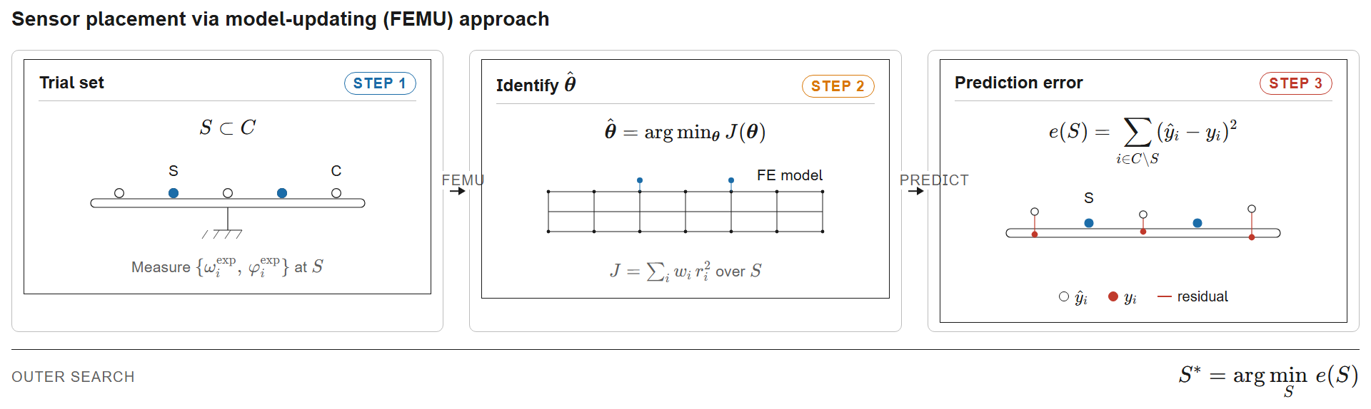
Figure 15:Model-updating (FEMU) approach for sensor placement. A trial sensor subset records modal data; an inverse problem identifies ; the identified model predicts responses at unmeasured locations and the prediction error is computed. The configuration with the lowest error is selected: .
5.4.2Force Identification Based Placement
A second approach evaluates sensor configurations by their ability to reconstruct unknown input forces. This is relevant for operational monitoring where external loads are not directly measured.
The method uses a simulation study. A known random force is applied to the finite element model and the acceleration response is recorded at all candidate sensor locations. For each candidate sensor subset, the original force is reconstructed from only those measurements using the structural model to invert from accelerations to input forces. Some sensor combinations allow accurate force recovery; others produce large errors. Testing many subsets identifies the configuration that minimizes the force identification error.
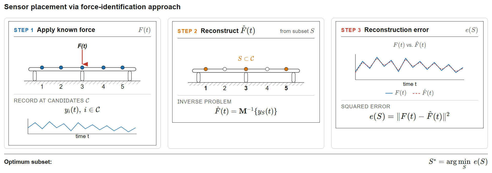
Figure 16:Force-identification approach for sensor placement. A known force is applied to the model and responses are recorded at all candidates . A sensor subset is used to solve the inverse problem , and the reconstructed force is compared against the true input via . The subset minimising this error, , is selected.
5.5Practical Considerations
The mathematically optimal sensor layout rarely translates directly to field conditions. Real structures impose constraints that algorithms cannot anticipate. Some locations may be inaccessible, too confined, or too dangerous for installation and maintenance. Power and data cables add cost and complexity. Some areas experience moisture, mechanical vibration, or electromagnetic interference that degrades signal quality.
Budget constraints matter as well. Fewer sensors reduce hardware and installation costs but may weaken monitoring capability. The practical approach is to begin with the theoretical optimum, then adjust individual locations to satisfy site requirements while preserving the overall spatial distribution. A sensor moved a short distance from its ideal position usually retains most of its information content.
Consulting site personnel during the design phase helps identify restrictions early. Experienced engineers know which areas are accessible, which surfaces suit sensor mounting, and where cables can be routed. Combining this knowledge with optimization results produces sensor networks that are both informative and maintainable.
6Conclusion
This chapter introduced optimization methods and their application to structural health monitoring. We began with finding extrema through derivatives, moved to gradient-based methods for multivariate functions, and showed how these techniques support system identification and finite element model updating. Gradient-free methods extended the treatment to discrete design spaces and non-differentiable objectives, with optimal sensor placement as the practical application.
Careful problem formulation and appropriate algorithm selection allow us to extract maximum information from limited sensor networks, calibrate complex models against measured data, and make defensible decisions about monitoring system design. These optimization techniques underpin many advanced SHM methodologies, including the machine learning approaches covered in the next chapter.
7Exercises
Solution to Exercise 1
import numpy as np
import matplotlib.pyplot as plt
from scipy.optimize import minimize

# Given data
L = 10.0  # m
A = 0.1   # m²
I = 0.001 # m⁴
f_measured = np.array([3.52, 22.03, 61.70])  # Hz

# Theoretical frequencies for cantilever beam
# λ_n L values for first three modes
lambda_L = np.array([1.875, 4.694, 7.855])

def compute_frequencies(E, rho):
    """Compute natural frequencies of cantilever beam"""
    frequencies = np.zeros(3)
    for i in range(3):
        frequencies[i] = (lambda_L[i]**2 / (2*np.pi*L**2)) * np.sqrt(E*I/(rho*A))
    return frequencies

def objective(params):
    """Objective function: sum of squared frequency errors"""
    E, rho = params
    if E <= 0 or rho <= 0:
        return 1e10

    f_predicted = compute_frequencies(E, rho)
    return np.sum((f_predicted - f_measured)**2 / f_measured**2)

# Initial guess
theta0 = [200e9, 7850]  # Steel-like properties

# Optimization
result = minimize(objective, theta0, method='L-BFGS-B',
                 bounds=[(1e9, 500e9), (100, 10000)])

E_opt, rho_opt = result.x
f_final = compute_frequencies(E_opt, rho_opt)

# Sensitivity analysis
delta = 0.01
dE = E_opt * delta
drho = rho_opt * delta

f_E_plus = compute_frequencies(E_opt + dE, rho_opt)
f_rho_plus = compute_frequencies(E_opt, rho_opt + drho)

sensitivity_E = (f_E_plus - f_final) / dE
sensitivity_rho = (f_rho_plus - f_final) / drho

# Results
print("="*60)
print("PARAMETER IDENTIFICATION RESULTS")
print("="*60)
print(f"Identified E = {E_opt/1e9:.2f} GPa")
print(f"Identified ρ = {rho_opt:.1f} kg/m³")
print(f"\nFrequency comparison:")
for i in range(3):
    error = abs(f_final[i] - f_measured[i]) / f_measured[i] * 100
    print(f"  Mode {i+1}: Measured = {f_measured[i]:.2f} Hz, "
          f"Predicted = {f_final[i]:.2f} Hz, Error = {error:.2f}%")

print(f"\nSensitivity analysis:")
print("  ∂f/∂E [Hz/Pa]:")
for i in range(3):
    print(f"    Mode {i+1}: {sensitivity_E[i]:.2e}")
print("  ∂f/∂ρ [Hz/(kg/m³)]:")
for i in range(3):
    print(f"    Mode {i+1}: {sensitivity_rho[i]:.2e}")

# Visualization
fig, axes = plt.subplots(1, 2, figsize=(12, 5))

# Frequency comparison
theta = np.arange(1, 4)
width = 0.35
axes[0].bar(theta - width/2, f_measured, width, label='Measured', color='#2E86AB')
axes[0].bar(theta + width/2, f_final, width, label='Identified', color='#F18F01')
axes[0].set_xlabel('Mode Number')
axes[0].set_ylabel('Frequency [Hz]')
axes[0].set_title('Frequency Comparison')
axes[0].set_xticks(theta)
axes[0].legend()
axes[0].grid(True, alpha=0.3)

# Sensitivity
sensitivity_norm_E = sensitivity_E * E_opt / f_final
sensitivity_norm_rho = sensitivity_rho * rho_opt / f_final

axes[1].plot(theta, sensitivity_norm_E, 'o-', linewidth=2, markersize=8,
            label='E sensitivity', color='#2E86AB')
axes[1].plot(theta, sensitivity_norm_rho, 's-', linewidth=2, markersize=8,
            label='ρ sensitivity', color='#F18F01')
axes[1].set_xlabel('Mode Number')
axes[1].set_ylabel('Normalized Sensitivity')
axes[1].set_title('Parameter Sensitivity')
axes[1].set_xticks(theta)
axes[1].legend()
axes[1].grid(True, alpha=0.3)

plt.tight_layout()
plt.show()
============================================================
PARAMETER IDENTIFICATION RESULTS
============================================================
Identified E = 200.00 GPa
Identified ρ = 4977.0 kg/m³
Frequency comparison:
Mode 1: Measured = 3.52 Hz, Predicted = 3.55 Hz, Error = 0.77%
Mode 2: Measured = 22.03 Hz, Predicted = 22.23 Hz, Error = 0.91%
Mode 3: Measured = 61.70 Hz, Predicted = 62.25 Hz, Error = 0.89%
Sensitivity analysis:
∂f/∂E [Hz/Pa]:
Mode 1: 8.85e-12
Mode 2: 5.54e-11
Mode 3: 1.55e-10
∂f/∂ρ [Hz/(kg/m³)]:
Mode 1: -3.54e-04
Mode 2: -2.22e-03
Mode 3: -6.21e-03
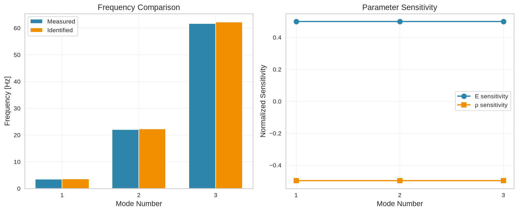
Discussion on identifiability: The two parameters affect frequencies differently. Young’s modulus appears in the numerator of the frequency equation, while density appears in the denominator, producing distinct sensitivity patterns. Higher modes carry more information but are also more sensitive to modeling errors. The condition number of the sensitivity matrix determines whether the parameters can be uniquely identified.
Solution to Exercise 2
import numpy as np
import matplotlib.pyplot as plt
from matplotlib.animation import FuncAnimation

class ParticleSwarmOptimization:
    def __init__(self, n_particles, n_dimensions, bounds, w=0.7, c1=1.5, c2=1.5):
        self.n_particles = n_particles
        self.n_dimensions = n_dimensions
        self.bounds = bounds
        self.w = w    # inertia weight
        self.c1 = c1  # cognitive parameter
        self.c2 = c2  # social parameter

        # Initialize particles
        self.positions = np.random.uniform(bounds[0], bounds[1],
                                          (n_particles, n_dimensions))
        self.velocities = np.random.uniform(-1, 1, (n_particles, n_dimensions))

        # Best positions
        self.pbest_positions = self.positions.copy()
        self.pbest_scores = np.full(n_particles, np.inf)
        self.gbest_position = None
        self.gbest_score = np.inf

        self.history = []

    def rastrigin(self, theta):
        """Rastrigin function"""
        n = len(theta)
        return 10*n + np.sum(theta**2 - 10*np.cos(2*np.pi*theta))

    def evaluate(self):
        """Evaluate all particles"""
        scores = np.array([self.rastrigin(pos) for pos in self.positions])

        # Update personal best
        better_mask = scores < self.pbest_scores
        self.pbest_scores[better_mask] = scores[better_mask]
        self.pbest_positions[better_mask] = self.positions[better_mask]

        # Update global best
        best_idx = np.argmin(scores)
        if scores[best_idx] < self.gbest_score:
            self.gbest_score = scores[best_idx]
            self.gbest_position = self.positions[best_idx].copy()

        return scores

    def update(self):
        """Update particle velocities and positions"""
        r1 = np.random.random((self.n_particles, self.n_dimensions))
        r2 = np.random.random((self.n_particles, self.n_dimensions))

        # Velocity update
        cognitive = self.c1 * r1 * (self.pbest_positions - self.positions)
        social = self.c2 * r2 * (self.gbest_position - self.positions)
        self.velocities = self.w * self.velocities + cognitive + social

        # Position update
        self.positions = self.positions + self.velocities

        # Boundary enforcement
        self.positions = np.clip(self.positions, self.bounds[0], self.bounds[1])

    def optimize(self, n_iterations):
        """Run PSO optimization"""
        for iteration in range(n_iterations):
            scores = self.evaluate()
            self.history.append({
                'iteration': iteration,
                'positions': self.positions.copy(),
                'gbest_score': self.gbest_score,
                'mean_score': np.mean(scores)
            })
            self.update()

        return self.gbest_position, self.gbest_score

# Run PSO with different swarm sizes
swarm_sizes = [10, 20, 40]
results = {}

for size in swarm_sizes:
    pso = ParticleSwarmOptimization(n_particles=size, n_dimensions=2,
                                   bounds=(-5.12, 5.12))
    best_pos, best_score = pso.optimize(100)
    results[size] = {
        'best_position': best_pos,
        'best_score': best_score,
        'history': pso.history
    }

# Visualization
fig, axes = plt.subplots(2, 2, figsize=(12, 10))

# Rastrigin function surface
theta_vals = np.linspace(-5.12, 5.12, 100)
THETA1, THETA2 = np.meshgrid(theta_vals, theta_vals)
Z = 10*2 + (THETA1**2 - 10*np.cos(2*np.pi*THETA1)) + (THETA2**2 - 10*np.cos(2*np.pi*THETA2))

axes[0, 0].contourf(THETA1, THETA2, Z, levels=50, cmap='RdYlBu_r', alpha=0.7)
axes[0, 0].set_xlabel('$\\theta_1$')
axes[0, 0].set_ylabel('$\\theta_2$')
axes[0, 0].set_title('Rastrigin Function')

# Final particle positions for different swarm sizes
colors = ['#F18F01', '#A23B72', '#2E86AB']
for i, (size, color) in enumerate(zip(swarm_sizes, colors)):
    final_positions = results[size]['history'][-1]['positions']
    axes[0, 0].scatter(final_positions[:, 0], final_positions[:, 1],
                      s=50, color=color, alpha=0.7, edgecolor='white',
                      label=f'{size} particles')

axes[0, 0].scatter(0, 0, s=200, color='red', marker='*',
                  edgecolor='white', linewidth=2, label='Global optimum')
axes[0, 0].legend()

# Convergence curves
for size, color in zip(swarm_sizes, colors):
    iterations = [h['iteration'] for h in results[size]['history']]
    gbest_scores = [h['gbest_score'] for h in results[size]['history']]
    axes[0, 1].semilogy(iterations, gbest_scores, linewidth=2.5,
                       color=color, label=f'{size} particles')

axes[0, 1].set_xlabel('Iteration')
axes[0, 1].set_ylabel('Best Score (log scale)')
axes[0, 1].set_title('Convergence Comparison')
axes[0, 1].legend()
axes[0, 1].grid(True, alpha=0.3)

# Effect of parameters
w_values = [0.4, 0.7, 0.9]
c1_values = [1.0, 1.5, 2.0]

for i, w in enumerate(w_values):
    pso = ParticleSwarmOptimization(n_particles=20, n_dimensions=2,
                                   bounds=(-5.12, 5.12), w=w)
    pso.optimize(100)
    iterations = [h['iteration'] for h in pso.history]
    gbest_scores = [h['gbest_score'] for h in pso.history]
    axes[1, 0].semilogy(iterations, gbest_scores, linewidth=2,
                       label=f'w = {w}', alpha=0.8)

axes[1, 0].set_xlabel('Iteration')
axes[1, 0].set_ylabel('Best Score (log scale)')
axes[1, 0].set_title('Effect of Inertia Weight')
axes[1, 0].legend()
axes[1, 0].grid(True, alpha=0.3)

for i, c1 in enumerate(c1_values):
    pso = ParticleSwarmOptimization(n_particles=20, n_dimensions=2,
                                   bounds=(-5.12, 5.12), c1=c1, c2=3-c1)
    pso.optimize(100)
    iterations = [h['iteration'] for h in pso.history]
    gbest_scores = [h['gbest_score'] for h in pso.history]
    axes[1, 1].semilogy(iterations, gbest_scores, linewidth=2,
                       label=f'c₁={c1}, c₂={3-c1}', alpha=0.8)

axes[1, 1].set_xlabel('Iteration')
axes[1, 1].set_ylabel('Best Score (log scale)')
axes[1, 1].set_title('Effect of Cognitive/Social Parameters')
axes[1, 1].legend()
axes[1, 1].grid(True, alpha=0.3)

plt.tight_layout()
plt.show()

# Print results
print("="*60)
print("PSO OPTIMIZATION RESULTS")
print("="*60)
for size in swarm_sizes:
    print(f"\nSwarm size: {size} particles")
    print(f"  Best position: {results[size]['best_position']}")
    print(f"  Best score: {results[size]['best_score']:.6f}")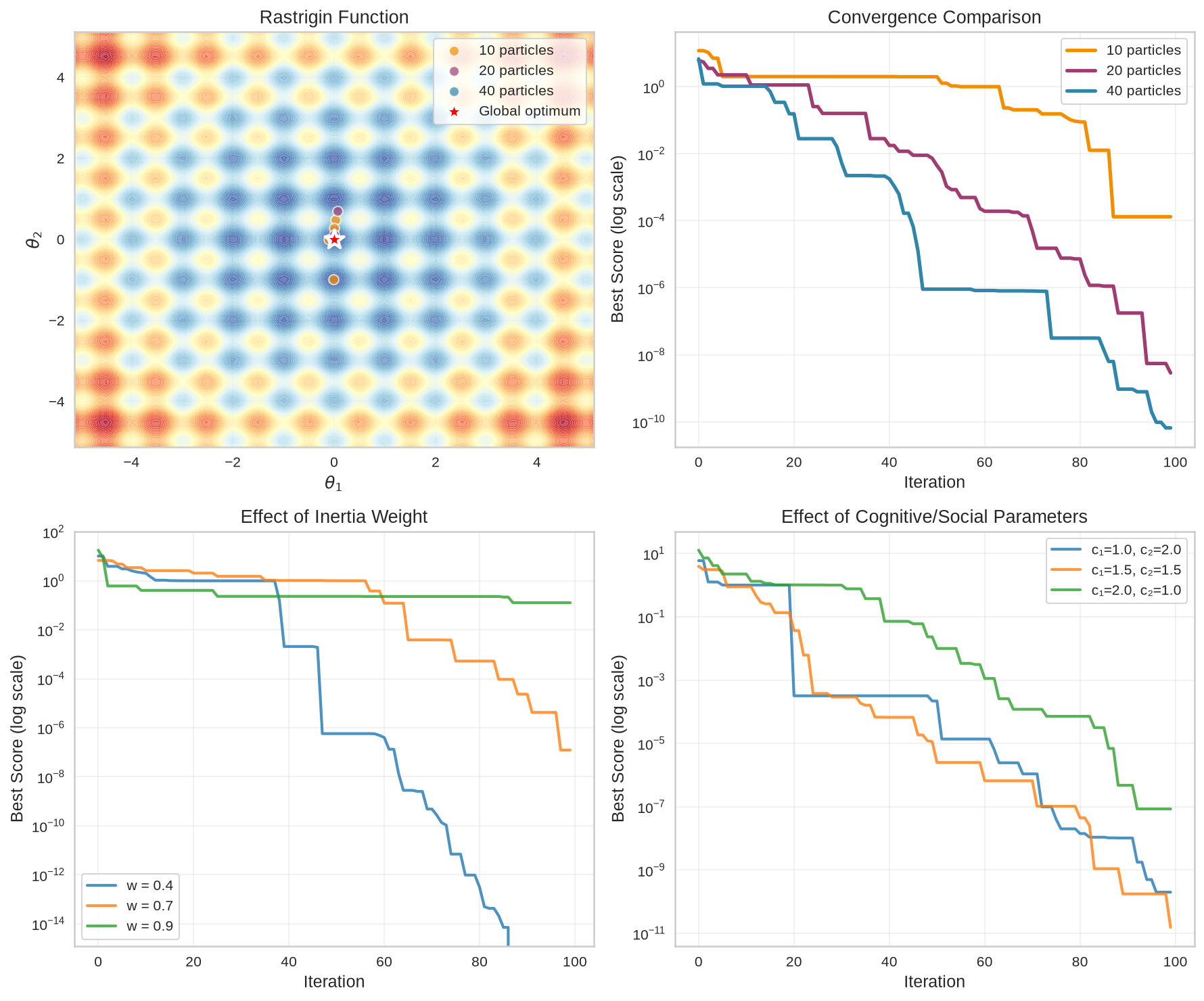
============================================================
PSO OPTIMIZATION RESULTS
============================================================

Swarm size: 10 particles
  Best position: [-0.0006301   0.00051956]
  Best score: 0.000132

Swarm size: 20 particles
  Best position: [ 3.52839703e-06 -1.42256157e-06]
  Best score: 0.000000

Swarm size: 40 particles
  Best position: [ 1.81969372e-07 -5.45573135e-07]
  Best score: 0.000000
Solution to Exercise 3
import numpy as np
import matplotlib.pyplot as plt
from scipy.linalg import eigh

# Building properties
n_floors = 3
n_dof = n_floors  # Horizontal displacement per floor
masses = np.array([100, 100, 80]) * 1000  # kg
stiffnesses = np.array([500, 450, 400]) * 1e6  # N/m

# Mass and stiffness matrices
M = np.diag(masses)
K = np.array([[stiffnesses[0] + stiffnesses[1], -stiffnesses[1], 0],
              [-stiffnesses[1], stiffnesses[1] + stiffnesses[2], -stiffnesses[2]],
              [0, -stiffnesses[2], stiffnesses[2]]])

# Modal analysis
eigenvalues, eigenvectors = eigh(K, M)
frequencies = np.sqrt(eigenvalues) / (2 * np.pi)
mode_shapes = eigenvectors

# Normalize mode shapes
for i in range(n_dof):
    mode_shapes[:, i] /= np.max(np.abs(mode_shapes[:, i]))

def effective_independence(mode_shapes, n_sensors):
    """Effective Independence method for sensor placement"""
    n_dof, n_modes = mode_shapes.shape
    n_sensors = min(n_sensors, n_dof)

    # Start with all candidate locations
    candidate_set = list(range(n_dof))
    selected_set = []

    # EI iterations
    while len(selected_set) < n_sensors:
        best_ei = 0
        best_candidate = None

        for candidate in candidate_set:
            if candidate not in selected_set:
                # Test configuration
                test_set = selected_set + [candidate]
                phi_s = mode_shapes[test_set, :]

                # Compute EI metric
                Q = phi_s @ phi_s.T
                try:
                    ei_metric = np.linalg.det(Q)
                except:
                    ei_metric = 0

                if ei_metric > best_ei:
                    best_ei = ei_metric
                    best_candidate = candidate

        if best_candidate is not None:
            selected_set.append(best_candidate)

    return sorted(selected_set)

def compute_mac(phi1, phi2):
    """Compute Modal Assurance Criterion"""
    n_modes1 = phi1.shape[1]
    n_modes2 = phi2.shape[1]
    mac = np.zeros((n_modes1, n_modes2))

    for i in range(n_modes1):
        for j in range(n_modes2):
            num = np.abs(np.dot(phi1[:, i], phi2[:, j]))**2
            den = np.dot(phi1[:, i], phi1[:, i]) * np.dot(phi2[:, j], phi2[:, j])
            mac[i, j] = num / den if den > 0 else 0

    return mac

# Test different numbers of sensors
sensor_configs = {}
for n_sensors in [1, 2, 3]:
    sensor_locations = effective_independence(mode_shapes, n_sensors)
    sensor_configs[n_sensors] = sensor_locations

# Visualization
fig, axes = plt.subplots(2, 2, figsize=(12, 10))

# Mode shapes
floor_heights = np.array([0, 3, 6, 9])  # m
colors = ['#2E86AB', '#F18F01', '#A23B72']

for i in range(n_dof):
    mode_disp = np.concatenate([[0], mode_shapes[:, i]])
    axes[0, 0].plot(mode_disp, floor_heights, 'o-', linewidth=2.5,
                   markersize=8, color=colors[i],
                   label=f'Mode {i+1} ({frequencies[i]:.2f} Hz)')

axes[0, 0].set_xlabel('Normalized Displacement')
axes[0, 0].set_ylabel('Height [m]')
axes[0, 0].set_title('Building Mode Shapes')
axes[0, 0].legend()
axes[0, 0].grid(True, alpha=0.3)
axes[0, 0].axhline(y=0, color='black', linewidth=2)

# Sensor configurations
for n_sensors, locations in sensor_configs.items():
    theta_pos = np.ones(n_floors) * (n_sensors * 0.3)
    y_pos = floor_heights[1:]

    # Building frame
    axes[0, 1].plot([n_sensors*0.3-0.15, n_sensors*0.3+0.15],
                   [floor_heights[i+1], floor_heights[i+1]],
                   'k-', linewidth=8, alpha=0.3)

    # Sensors
    sensor_y = floor_heights[1:][locations]
    axes[0, 1].scatter([n_sensors*0.3]*len(locations), sensor_y,
                      s=200, color=colors[n_sensors-1], marker='s',
                      edgecolor='white', linewidth=2)

    # Labels
    axes[0, 1].text(n_sensors*0.3, -1, f'{n_sensors} sensor{"s" if n_sensors > 1 else ""}',
                   ha='center', fontsize=10)

axes[0, 1].set_xlim([0, 1.2])
axes[0, 1].set_ylim([-2, 10])
axes[0, 1].set_ylabel('Height [m]')
axes[0, 1].set_title('Sensor Configurations')
axes[0, 1].set_xticks([])
axes[0, 1].axhline(y=0, color='black', linewidth=2)

# MAC matrices
for idx, (n_sensors, locations) in enumerate([(2, sensor_configs[2]),
                                              (3, sensor_configs[3])]):
    phi_full = mode_shapes
    phi_measured = mode_shapes[locations, :]

    # Mode shape expansion using pseudo-inverse
    # phi_measured: (n_sensors, n_modes), phi_full: (n_dof, n_modes)
    # We want to find phi_expanded: (n_dof, n_modes) from partial measurements

    # Correct formula: phi_expanded = phi_full @ phi_measured.T @ pinv(phi_measured @ phi_measured.T)
    phi_measured_T = phi_measured.T  # (n_modes, n_sensors)
    gram_matrix = phi_measured @ phi_measured_T  # (n_sensors, n_sensors)

    try:
        phi_expanded = phi_full @ phi_measured_T @ np.linalg.pinv(gram_matrix)
        phi_expanded = phi_expanded @ phi_measured  # (n_dof, n_modes)
    except (np.linalg.LinAlgError, ValueError) as e:
        # Fallback: use regularized pseudo-inverse or simple reconstruction
        try:
            reg_factor = 1e-6 * np.trace(gram_matrix) / gram_matrix.shape[0]
            gram_reg = gram_matrix + reg_factor * np.eye(gram_matrix.shape[0])
            phi_expanded = phi_full @ phi_measured_T @ np.linalg.inv(gram_reg)
            phi_expanded = phi_expanded @ phi_measured
        except (np.linalg.LinAlgError, ValueError):
            # Ultimate fallback: use simple interpolation
            print(f"Matrix operation failed for {n_sensors} sensors, using simple reconstruction")
            phi_expanded = np.copy(phi_full)  # Use full mode shapes as fallback

    mac = compute_mac(phi_full, phi_expanded)

    ax = axes[1, idx]
    im = ax.imshow(mac, cmap='RdYlBu_r', vmin=0, vmax=1, aspect='equal')
    ax.set_xlabel('Reconstructed Mode')
    ax.set_ylabel('True Mode')
    ax.set_title(f'MAC Matrix ({n_sensors} sensors)')
    ax.set_xticks(range(n_dof))
    ax.set_yticks(range(n_dof))
    ax.set_xticklabels([f'{i+1}' for i in range(n_dof)])
    ax.set_yticklabels([f'{i+1}' for i in range(n_dof)])

    # Add text annotations
    for i in range(n_dof):
        for j in range(n_dof):
            ax.text(j, i, f'{mac[i,j]:.2f}', ha='center', va='center',
                   color='white' if mac[i,j] < 0.5 else 'black')

    plt.colorbar(im, ax=ax)

plt.tight_layout()
plt.show()

# Print results
print("="*60)
print("EFFECTIVE INDEPENDENCE SENSOR PLACEMENT")
print("="*60)
for n_sensors, locations in sensor_configs.items():
    print(f"\n{n_sensors} Sensor{'s' if n_sensors > 1 else ''}:")
    floors = [f"Floor {loc+1}" for loc in locations]
    print(f"  Locations: {', '.join(floors)}")

    # Compute observability metric
    phi_s = mode_shapes[locations, :]
    Q = phi_s @ phi_s.T
    det_Q = np.linalg.det(Q) if len(locations) <= n_dof else 0
    print(f"  Determinant of Q: {det_Q:.4e}")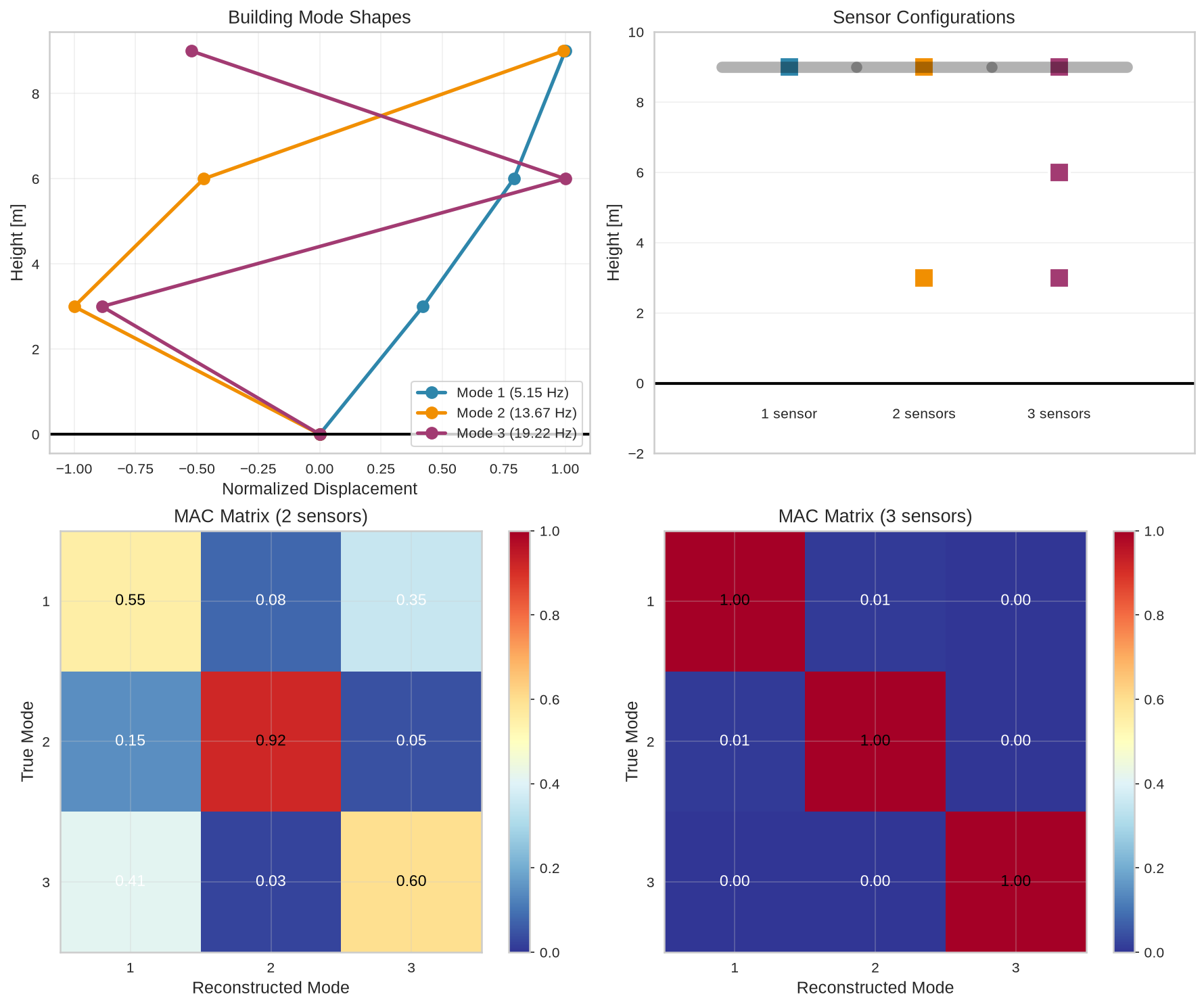
============================================================
EFFECTIVE INDEPENDENCE SENSOR PLACEMENT
============================================================

1 Sensor:
  Locations: Floor 3
  Determinant of Q: 2.2577e+00

2 Sensors:
  Locations: Floor 1, Floor 3
  Determinant of Q: 4.4195e+00

3 Sensors:
  Locations: Floor 1, Floor 2, Floor 3
  Determinant of Q: 8.0701e+00
Solution to Exercise 4
import numpy as np
from scipy.optimize import minimize
import matplotlib.pyplot as plt
import time

def rosenbrock(theta):
    """Rosenbrock function"""
    return np.sum(100*(theta[1:] - theta[:-1]**2)**2 + (1 - theta[:-1])**2)

def rosenbrock_gradient(theta):
    """Gradient of Rosenbrock function"""
    n = len(theta)
    grad = np.zeros(n)

    for i in range(n-1):
        grad[i] += -400 * theta[i] * (theta[i+1] - theta[i]**2) - 2 * (1 - theta[i])
        grad[i+1] += 200 * (theta[i+1] - theta[i]**2)

    return grad

class GeneticAlgorithm:
    def __init__(self, pop_size, n_vars, bounds, mutation_rate=0.1, crossover_rate=0.8):
        self.pop_size = pop_size
        self.n_vars = n_vars
        self.bounds = bounds
        self.mutation_rate = mutation_rate
        self.crossover_rate = crossover_rate

    def initialize_population(self):
        """Initialize random population"""
        return np.random.uniform(self.bounds[0], self.bounds[1],
                               (self.pop_size, self.n_vars))

    def selection(self, population, fitness):
        """Tournament selection"""
        selected = []
        for _ in range(self.pop_size):
            i, j = np.random.choice(self.pop_size, 2, replace=False)
            selected.append(population[i] if fitness[i] < fitness[j] else population[j])
        return np.array(selected)

    def crossover(self, parent1, parent2):
        """Arithmetic crossover"""
        if np.random.random() < self.crossover_rate:
            alpha = np.random.random()
            child1 = alpha * parent1 + (1 - alpha) * parent2
            child2 = (1 - alpha) * parent1 + alpha * parent2
            return child1, child2
        return parent1.copy(), parent2.copy()

    def mutation(self, individual):
        """Gaussian mutation"""
        if np.random.random() < self.mutation_rate:
            mutation_strength = 0.1 * (self.bounds[1] - self.bounds[0])
            individual += np.random.normal(0, mutation_strength, self.n_vars)
            individual = np.clip(individual, self.bounds[0], self.bounds[1])
        return individual

    def optimize(self, objective, n_generations):
        """Run genetic algorithm"""
        population = self.initialize_population()
        history = []

        for generation in range(n_generations):
            # Evaluate fitness
            fitness = np.array([objective(ind) for ind in population])
            best_idx = np.argmin(fitness)

            history.append({
                'generation': generation,
                'best_fitness': fitness[best_idx],
                'mean_fitness': np.mean(fitness),
                'best_individual': population[best_idx].copy()
            })

            # Selection
            selected = self.selection(population, fitness)

            # Crossover and mutation
            offspring = []
            for i in range(0, self.pop_size, 2):
                parent1 = selected[i]
                parent2 = selected[min(i+1, self.pop_size-1)]

                child1, child2 = self.crossover(parent1, parent2)
                child1 = self.mutation(child1)
                child2 = self.mutation(child2)

                offspring.extend([child1, child2])

            population = np.array(offspring[:self.pop_size])

        return history

class HybridOptimizer:
    def __init__(self, ga_generations=50, local_search_budget=100):
        self.ga_generations = ga_generations
        self.local_search_budget = local_search_budget

    def optimize(self, objective, gradient, n_vars, bounds):
        """Hybrid GA + Local Search"""
        # Phase 1: Global search with GA
        ga = GeneticAlgorithm(pop_size=50, n_vars=n_vars, bounds=bounds)
        ga_history = ga.optimize(objective, self.ga_generations)

        # Get best solution from GA
        ga_best = ga_history[-1]['best_individual']

        # Phase 2: Local refinement
        result = minimize(objective, ga_best, method='L-BFGS-B',
                         jac=gradient, bounds=[(bounds[0], bounds[1])]*n_vars,
                         options={'maxfun': self.local_search_budget})

        return {
            'ga_history': ga_history,
            'ga_best': ga_best,
            'final_solution': result.x,
            'final_value': result.fun,
            'local_search_success': result.success
        }

# Run experiments
n_vars = 10
bounds = (-5, 5)
n_runs = 5

methods = {
    'GA Only': lambda: GeneticAlgorithm(pop_size=50, n_vars=n_vars, bounds=bounds).optimize(rosenbrock, 100),
    'Local Only': lambda: minimize(rosenbrock, np.random.uniform(-5, 5, n_vars),
                                  method='L-BFGS-B', jac=rosenbrock_gradient,
                                  bounds=[bounds]*n_vars, options={'maxfun': 1000}),
    'Hybrid': lambda: HybridOptimizer(ga_generations=50, local_search_budget=500).optimize(
                      rosenbrock, rosenbrock_gradient, n_vars, bounds)
}

results = {method: [] for method in methods}

for run in range(n_runs):
    print(f"Run {run+1}/{n_runs}")

    for method_name, method_func in methods.items():
        start_time = time.time()

        if method_name == 'GA Only':
            history = method_func()
            best_value = history[-1]['best_fitness']
            best_solution = history[-1]['best_individual']
        elif method_name == 'Local Only':
            result = method_func()
            best_value = result.fun
            best_solution = result.x
        else:  # Hybrid
            hybrid_result = method_func()
            best_value = hybrid_result['final_value']
            best_solution = hybrid_result['final_solution']

        elapsed_time = time.time() - start_time

        results[method_name].append({
            'value': best_value,
            'solution': best_solution,
            'time': elapsed_time
        })

# Analysis
fig, axes = plt.subplots(2, 2, figsize=(12, 10))

# Performance comparison
method_names = list(methods.keys())
mean_values = [np.mean([r['value'] for r in results[m]]) for m in method_names]
std_values = [np.std([r['value'] for r in results[m]]) for m in method_names]

axes[0, 0].bar(method_names, mean_values, yerr=std_values,
              color=['#2E86AB', '#F18F01', '#A23B72'], capsize=5)
axes[0, 0].set_ylabel('Objective Value')
axes[0, 0].set_title('Optimization Performance (Mean ± Std)')
axes[0, 0].set_yscale('log')

# Time comparison
mean_times = [np.mean([r['time'] for r in results[m]]) for m in method_names]
axes[0, 1].bar(method_names, mean_times,
              color=['#2E86AB', '#F18F01', '#A23B72'])
axes[0, 1].set_ylabel('Time [seconds]')
axes[0, 1].set_title('Computational Time')

# Convergence history (for one run)
ga_history = GeneticAlgorithm(pop_size=50, n_vars=n_vars, bounds=bounds).optimize(rosenbrock, 100)
hybrid_result = HybridOptimizer(ga_generations=50, local_search_budget=500).optimize(
                rosenbrock, rosenbrock_gradient, n_vars, bounds)

generations = [h['generation'] for h in ga_history]
ga_best = [h['best_fitness'] for h in ga_history]
hybrid_ga = [h['best_fitness'] for h in hybrid_result['ga_history']]

axes[1, 0].semilogy(generations[:50], hybrid_ga, linewidth=2.5,
                   color='#A23B72', label='Hybrid (GA phase)')
axes[1, 0].semilogy(generations, ga_best, linewidth=2.5,
                   color='#2E86AB', label='GA Only')
axes[1, 0].axvline(x=50, color='gray', linestyle='--', alpha=0.5)
axes[1, 0].text(52, hybrid_ga[-1], 'Local search\nstarts', fontsize=9)
axes[1, 0].set_xlabel('Generation')
axes[1, 0].set_ylabel('Best Fitness (log scale)')
axes[1, 0].set_title('Convergence Comparison')
axes[1, 0].legend()
axes[1, 0].grid(True, alpha=0.3)

# Success rate
success_threshold = 10.0
success_rates = []
for method_name in method_names:
    successes = sum(1 for r in results[method_name] if r['value'] < success_threshold)
    success_rates.append(100 * successes / n_runs)

axes[1, 1].bar(method_names, success_rates,
              color=['#2E86AB', '#F18F01', '#A23B72'])
axes[1, 1].set_ylabel('Success Rate [%]')
axes[1, 1].set_title(f'Success Rate (threshold = {success_threshold})')

plt.tight_layout()
plt.show()

# Print detailed results
print("="*60)
print("HYBRID OPTIMIZATION RESULTS")
print("="*60)
for method_name in method_names:
    values = [r['value'] for r in results[method_name]]
    times = [r['time'] for r in results[method_name]]

    print(f"\n{method_name}:")
    print(f"  Best value: {np.min(values):.6f}")
    print(f"  Mean value: {np.mean(values):.6f} ± {np.std(values):.6f}")
    print(f"  Mean time: {np.mean(times):.3f} seconds")
    print(f"  Success rate: {success_rates[method_names.index(method_name)]:.1f}%")
Run 1/5
Run 2/5
Run 3/5
Run 4/5
Run 5/5
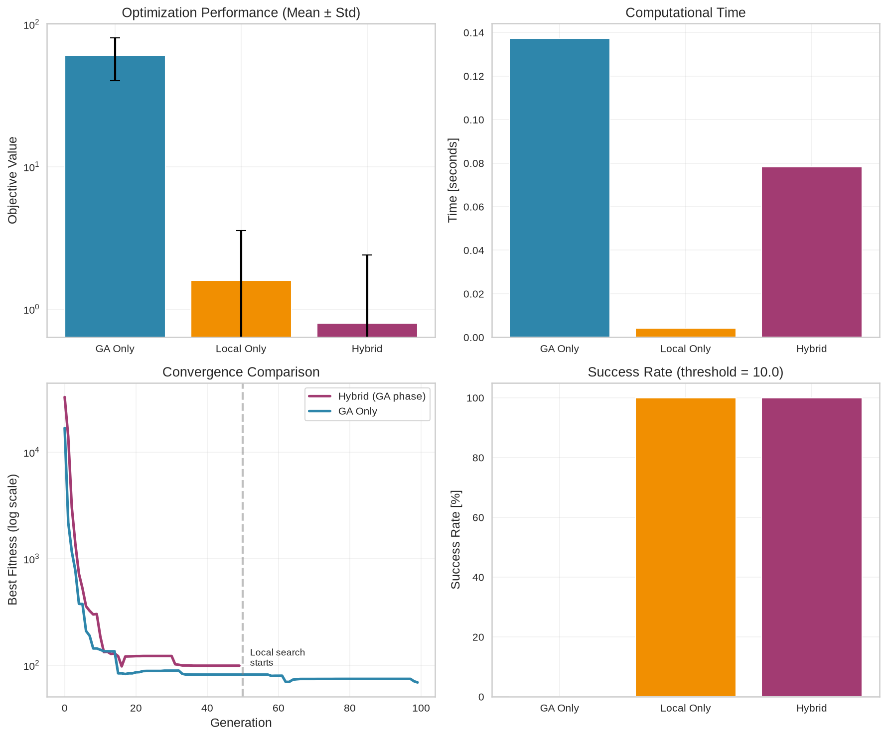
============================================================
HYBRID OPTIMIZATION RESULTS
============================================================

GA Only:
  Best value: 30.673519
  Mean value: 60.224720 ± 20.146828
  Mean time: 0.137 seconds
  Success rate: 0.0%

Local Only:
  Best value: 0.000000
  Mean value: 1.594632 ± 1.953017
  Mean time: 0.004 seconds
  Success rate: 100.0%

Hybrid:
  Best value: 0.000000
  Mean value: 0.797316 ± 1.594632
  Mean time: 0.078 seconds
  Success rate: 100.0%
Solution to Exercise 5
import numpy as np
from scipy.linalg import eigh
from scipy.optimize import differential_evolution
import matplotlib.pyplot as plt

class DamagedBeamModel:
    def __init__(self, n_elements=20, length=10.0):
        self.n_elements = n_elements
        self.length = length
        self.element_length = length / n_elements
        self.E = 200e9  # Pa
        self.I = 1e-4   # m^4
        self.rho = 7850  # kg/m^3
        self.A = 0.01   # m^2

    def assemble_matrices(self, damage_pattern):
        """Assemble mass and stiffness matrices with damage"""
        n_dof = self.n_elements + 1
        K = np.zeros((n_dof, n_dof))
        M = np.zeros((n_dof, n_dof))

        L = self.element_length

        for i in range(self.n_elements):
            # Stiffness reduction due to damage
            damage_factor = 1.0 - damage_pattern[i]
            k_elem = (self.E * self.I * damage_factor / L**3) * np.array([
                [12, -12],
                [-12, 12]
            ])

            m_elem = (self.rho * self.A * L / 6) * np.array([
                [2, 1],
                [1, 2]
            ])

            # Assembly
            K[i:i+2, i:i+2] += k_elem
            M[i:i+2, i:i+2] += m_elem

        return K, M

    def modal_analysis(self, damage_pattern):
        """Compute natural frequencies and mode shapes"""
        K, M = self.assemble_matrices(damage_pattern)

        # Apply simply supported boundary conditions
        # Remove first and last DOFs
        K_bc = K[1:-1, 1:-1]
        M_bc = M[1:-1, 1:-1]

        # Solve eigenvalue problem
        eigenvalues, eigenvectors = eigh(K_bc, M_bc)
        frequencies = np.sqrt(eigenvalues) / (2 * np.pi)

        # Expand mode shapes to include boundary conditions
        n_modes = len(frequencies)
        mode_shapes = np.zeros((self.n_elements + 1, n_modes))
        mode_shapes[1:-1, :] = eigenvectors

        return frequencies, mode_shapes

# Generate synthetic damaged beam data
true_damage = np.zeros(20)
true_damage[7:10] = 0.3   # 30% damage in elements 8-10
true_damage[15] = 0.2      # 20% damage in element 16

beam = DamagedBeamModel()
true_freq, true_modes = beam.modal_analysis(true_damage)

# Add measurement noise
noise_level = 0.02
measured_freq = true_freq[:5] * (1 + noise_level * np.random.randn(5))

def objective_function(damage_params, beam_model, measured_data):
    """Objective function for damage identification"""
    # Ensure damage values are between 0 and 1
    damage_pattern = np.clip(damage_params, 0, 0.8)

    # Compute predicted frequencies
    predicted_freq, _ = beam_model.modal_analysis(damage_pattern)

    # Frequency error
    n_modes = len(measured_data)
    freq_error = np.sum(((predicted_freq[:n_modes] - measured_data) / measured_data)**2)

    # Regularization (prefer sparse damage)
    sparsity_penalty = 0.01 * np.sum(damage_pattern)

    return freq_error + sparsity_penalty

# Optimization
bounds = [(0, 0.8) for _ in range(beam.n_elements)]

result = differential_evolution(
    objective_function,
    bounds,
    args=(beam, measured_freq),
    maxiter=200,
    popsize=15,
    seed=42,
    polish=True
)

identified_damage = result.x
identified_freq, _ = beam.modal_analysis(identified_damage)

# Noise sensitivity analysis
noise_levels = [0.01, 0.02, 0.05, 0.1]
identification_errors = []

for noise in noise_levels:
    noisy_freq = true_freq[:5] * (1 + noise * np.random.randn(5))

    result_noise = differential_evolution(
        objective_function,
        bounds,
        args=(beam, noisy_freq),
        maxiter=100,
        popsize=15,
        seed=42
    )

    damage_error = np.mean(np.abs(result_noise.x - true_damage))
    identification_errors.append(damage_error)

# Visualization
fig, axes = plt.subplots(2, 2, figsize=(14, 10))

# Damage comparison
element_positions = np.arange(1, beam.n_elements + 1)
width = 0.4

axes[0, 0].bar(element_positions - width/2, true_damage, width,
              label='True Damage', color='#2E86AB')
axes[0, 0].bar(element_positions + width/2, identified_damage, width,
              label='Identified Damage', color='#F18F01')
axes[0, 0].set_xlabel('Element Number')
axes[0, 0].set_ylabel('Damage Level')
axes[0, 0].set_title('Damage Identification Results')
axes[0, 0].legend()
axes[0, 0].grid(True, alpha=0.3, axis='y')

# Frequency comparison
mode_numbers = np.arange(1, 6)
axes[0, 1].plot(mode_numbers, true_freq[:5], 'o-', linewidth=2.5,
               markersize=8, label='True', color='#2E86AB')
axes[0, 1].plot(mode_numbers, measured_freq, 's', markersize=8,
               label='Measured', color='gray')
axes[0, 1].plot(mode_numbers, identified_freq[:5], '^-', linewidth=2.5,
               markersize=8, label='Identified', color='#F18F01')
axes[0, 1].set_xlabel('Mode Number')
axes[0, 1].set_ylabel('Frequency [Hz]')
axes[0, 1].set_title('Frequency Comparison')
axes[0, 1].legend()
axes[0, 1].grid(True, alpha=0.3)

# Damage pattern along beam
theta_positions = np.linspace(0, beam.length, beam.n_elements + 1)
theta_centers = (theta_positions[:-1] + theta_positions[1:]) / 2

axes[1, 0].fill_between(theta_centers, 0, true_damage, alpha=0.5,
                       label='True Damage', color='#2E86AB', step='mid')
axes[1, 0].fill_between(theta_centers, 0, -identified_damage, alpha=0.5,
                       label='Identified Damage', color='#F18F01', step='mid')
axes[1, 0].set_xlabel('Position along beam [m]')
axes[1, 0].set_ylabel('Damage Level')
axes[1, 0].set_title('Spatial Damage Distribution')
axes[1, 0].legend()
axes[1, 0].grid(True, alpha=0.3)
axes[1, 0].axhline(y=0, color='black', linewidth=0.5)

# Noise sensitivity
axes[1, 1].plot(np.array(noise_levels)*100, np.array(identification_errors)*100,
               'o-', linewidth=2.5, markersize=8, color='#A23B72')
axes[1, 1].set_xlabel('Noise Level [%]')
axes[1, 1].set_ylabel('Mean Identification Error [%]')
axes[1, 1].set_title('Effect of Measurement Noise')
axes[1, 1].grid(True, alpha=0.3)

plt.tight_layout()
plt.show()

# Print results
print("="*60)
print("DAMAGE IDENTIFICATION RESULTS")
print("="*60)
print(f"Optimization converged: {result.success}")
print(f"Final objective value: {result.fun:.6f}")

print("\nDamage identification accuracy:")
for i in range(beam.n_elements):
    if true_damage[i] > 0.05 or identified_damage[i] > 0.05:
        print(f"  Element {i+1}: True = {true_damage[i]:.2f}, "
              f"Identified = {identified_damage[i]:.2f}, "
              f"Error = {abs(true_damage[i]-identified_damage[i])*100:.1f}%")

print("\nNoise sensitivity analysis:")
for noise, error in zip(noise_levels, identification_errors):
    print(f"  {noise*100:.0f}% noise → {error*100:.1f}% identification error")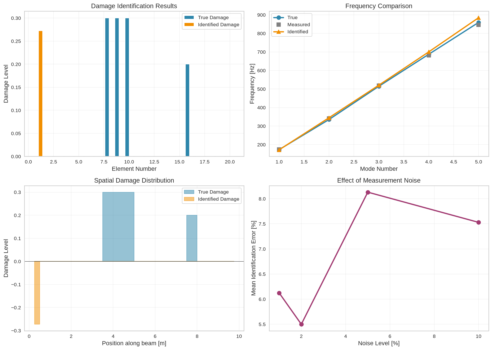
============================================================
DAMAGE IDENTIFICATION RESULTS
============================================================
Optimization converged: False
Final objective value: 0.005895

Damage identification accuracy:
  Element 1: True = 0.00, Identified = 0.27, Error = 27.3%
  Element 8: True = 0.30, Identified = 0.00, Error = 30.0%
  Element 9: True = 0.30, Identified = 0.00, Error = 30.0%
  Element 10: True = 0.30, Identified = 0.00, Error = 30.0%
  Element 16: True = 0.20, Identified = 0.00, Error = 20.0%

Noise sensitivity analysis:
  1% noise → 6.1% identification error
  2% noise → 5.5% identification error
  5% noise → 8.1% identification error
  10% noise → 7.5% identification error