Chapter 8: Advanced Parametric System Identification and Time-Series Forecasting

1Overview¶

Throughout this book, we have built a complete toolkit for structural health monitoring: from understanding sensor hardware and signal conditioning (Chapters 1 and 2), through time-domain and frequency-domain analysis (Chapters 3 and 4), to feature extraction and anomaly detection (Chapter 5), finite element model updating and optimal sensor placement (Chapter 6), and machine learning classification (Chapter 7). Each of these tools addresses a particular stage of the monitoring pipeline. In this final chapter, we bring together many of these ideas under a single mathematical framework: parametric time-series models and optimal state estimation.

The central question motivating this chapter is practical. Suppose a bridge is instrumented with a handful of accelerometers, yet engineers need displacement estimates at locations where no sensor exists. Or suppose that an autonomous monitoring system must distinguish genuine structural damage from ordinary fluctuations in traffic loading. Non-parametric spectral methods such as the FFT treat each frequency bin independently and cannot easily address these problems. Parametric models, by contrast, encode the physics of structural vibration into a small set of coefficients, and from those coefficients we can extract natural frequencies, predict future response, fuse measurements from multiple sensor types, and quantify uncertainty in every estimate.

This chapter develops five progressively richer model families. We begin with autoregressive (AR) models, the simplest parametric representation of vibration data, and show how their coefficients map directly to modal parameters. We then extend to ARMA models, which account for colored excitation, and to ARMAX models, which incorporate measured inputs such as traffic loads or wind speed. The transition to state-space representations reformulates the problem in matrix form, enabling multi-input multi-output analysis and setting the stage for the Kalman filter, an optimal recursive algorithm that fuses physics-based predictions with noisy sensor data to produce real-time state estimates with quantified uncertainty.

Learning Objectives:

Derive stability conditions and extract modal parameters (natural frequencies, damping ratios) from AR, ARMA, and ARMAX models
Construct state-space representations directly from structural equations of motion
Implement Kalman filters for optimal state estimation, virtual sensing, and real-time damage detection
Validate parametric models through residual diagnostics, information criteria, and physical plausibility checks
Select the appropriate model family for a given monitoring scenario based on data availability and objectives

2Motivation: From Spectra to Parametric Models¶

Non-parametric spectral methods such as the periodogram and Welch’s method, covered in Chapter 4, estimate power spectral density by treating each frequency bin as an independent quantity. For a signal sampled at $f_s$ Hz over $N$ points, the FFT produces $N/2$ spectral coefficients, each describing the energy content at one frequency. This approach is straightforward and widely used, but it has three limitations that become significant in real-time SHM applications.

First, spectral resolution is inversely proportional to record length, so short monitoring windows yield broad, poorly resolved peaks that obscure closely spaced modes. Second, the FFT provides no mechanism for predicting future response or for fusing data from different sensor types into a unified state estimate. Third, each spectral bin is estimated independently, so the total number of parameters equals the number of frequency bins, which is far more than the handful of physical modes that actually govern the response.

Parametric models address all three limitations. A few AR coefficients can capture multi-modal dynamics with high frequency resolution even from short records, because the model enforces the physical constraint that structural vibration consists of damped sinusoids. The coefficients map directly to natural frequencies and damping ratios through well-defined transformations, giving every parameter a physical interpretation. And because the model is compact, it is suitable for real-time processing and statistical inference with rigorous uncertainty bounds.

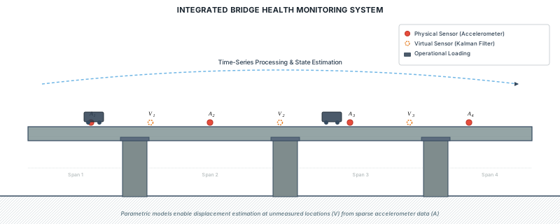
Figure 1:Integrated bridge health monitoring system showing physical accelerometers (red circles) and virtual sensing locations (dashed orange circles) estimated via Kalman filtering from parametric time-series models. Traffic loading provides operational excitation while parametric models enable displacement estimation at uninstrumented spans.

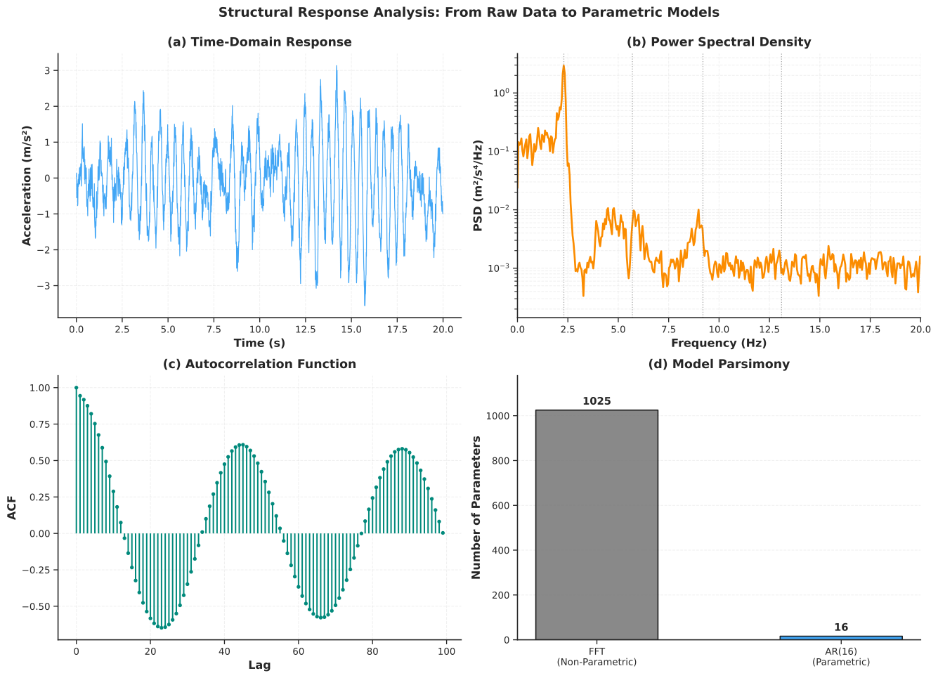
Figure 2:Structural response analysis: from raw data to parametric models. (a) Time-domain acceleration response of a simulated bridge with four vibration modes. (b) Power spectral density revealing modal peaks. (c) Autocorrelation function showing persistent oscillatory structure. (d) Model parsimony comparison between non-parametric FFT and parametric AR(16) representations.

The figure above illustrates the core idea. Panel (a) shows a simulated bridge acceleration record containing four vibration modes with damping ratios between 1.8% and 4.5%. Panel (b) reveals these modes as peaks in the power spectral density, estimated using Welch’s method. Panel (c) shows the autocorrelation function, which decays slowly because the signal is dominated by lightly damped oscillatory components. Panel (d) highlights the key advantage of parametric modeling: the FFT requires over a thousand coefficients to represent the spectrum, whereas an AR(16) model captures the same four modes with only 16 coefficients. This parsimony is not just a matter of storage; it reflects the physical reality that a bridge’s vibration is governed by a small number of modes, and a good model should encode that structure directly.

3Autoregressive (AR) Models¶

3.1From Vibration Memory to Mathematical Prediction¶

When a truck crosses a bridge, the resulting vibration does not vanish instantly. Instead, the bridge oscillates at its natural frequencies, with each cycle slightly smaller than the last because of damping. This gradual decay means that the current vibration depends strongly on the recent past: the bridge has memory. Autoregressive models exploit this memory by expressing the current measurement as a weighted combination of previous measurements plus a random innovation term that represents unmeasured ambient excitation such as wind gusts and distant traffic.

AR models are the natural starting point for parametric SHM because they require only output measurements (no force or input data), they can be estimated by solving a linear system, and their coefficients encode the modal parameters of the structure through a well-defined mapping. In practice, AR-based modal identification is widely used for ambient vibration testing of bridges, buildings, and wind turbines, where the excitation cannot be measured directly.

AR models are most effective for stationary, lightly damped, linear structures under ambient excitation. They are well suited to output-only monitoring of civil infrastructure such as bridges and buildings, where operational loads vary slowly relative to the structural dynamics. They are less appropriate for structures exhibiting strong nonlinearity (large deformations, impacts) or for situations where the structural properties change rapidly during the measurement window.

3.2Mathematical Framework¶

An AR( $p$ ) model expresses the current observation as a linear combination of $p$ past values plus an innovation (white noise) term:

x_t = \sum_{i=1}^{p} \phi_i x_{t-i} + \varepsilon_t, \quad \varepsilon_t \sim \mathcal{N}(0, \sigma^2)

(1)

where $x_t$ is the measured response at time $t$ (for example, acceleration or displacement), $\phi_i$ are the AR coefficients that encode the structural dynamics, $p$ is the model order (the number of past values used), and $\varepsilon_t$ is the innovation, a zero-mean white noise process with variance $\sigma^2$ representing unmeasured excitation.

The AR model admits two equivalent representations that are useful for different purposes. The polynomial form facilitates pole extraction:

A(z) x_t = \varepsilon_t, \quad \text{where } A(z) = 1 - \sum_{i=1}^{p}\phi_i z^{-i}

(2)

The transfer function form reveals the frequency response:

H(z) = \frac{1}{A(z)} = \frac{1}{1 - \phi_1 z^{-1} - \phi_2 z^{-2} - \cdots - \phi_p z^{-p}}

(3)

The roots of the characteristic polynomial $A(z) = 0$ are the poles of the system, and for stability all poles must lie strictly inside the unit circle in the complex $z$ -plane: $|\lambda_i| < 1$ for every pole $\lambda_i$ .

AR(p) model block diagram showing the feedback structure with delay operators z^{-1}, autoregressive coefficients \phi_i, and white-noise innovation \varepsilon_t \sim \mathcal{N}(0, \sigma_\varepsilon^2). The recursion y_t = \phi_1 y_{t-1} + \phi_2 y_{t-2} + \cdots + \phi_p y_{t-p} + \varepsilon_t links the system’s memory (past values) to its current output; the characteristic-polynomial roots (poles) map directly to continuous-time structural modal parameters through the logarithmic transformation described below. 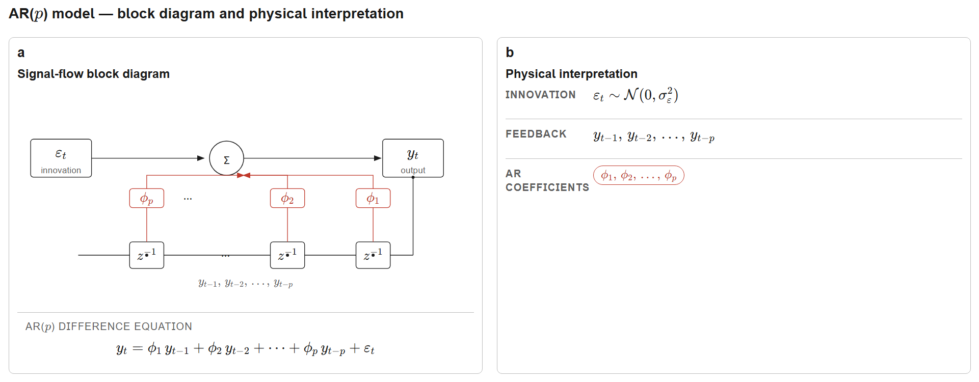— Figure 3:AR( $p$ ) model block diagram showing the feedback structure with delay operators $z^{-1}$ , autoregressive coefficients $\phi_i$ , and white-noise innovation $\varepsilon_t \sim \mathcal{N}(0, \sigma_\varepsilon^2)$ . The recursion $y_t = \phi_1 y_{t-1} + \phi_2 y_{t-2} + \cdots + \phi_p y_{t-p} + \varepsilon_t$ links the system’s memory (past values) to its current output; the characteristic-polynomial roots (poles) map directly to continuous-time structural modal parameters through the logarithmic transformation described below.

The connection between discrete-time AR poles and continuous-time structural modes is the key result that makes AR models physically meaningful. For a discrete-time pole $\lambda = r e^{j\theta}$ obtained from a model sampled at interval $\Delta t$ , the corresponding continuous-time modal parameters are:

\omega_n = \frac{\sqrt{(\ln r)^2 + \theta^2}}{\Delta t}, \quad \zeta = -\frac{\ln r}{\sqrt{(\ln r)^2 + \theta^2}}, \quad f_n = \frac{\omega_n}{2\pi}

(4)

where $\omega_n$ is the natural frequency in rad/s, $\zeta$ is the dimensionless damping ratio, $f_n$ is the natural frequency in Hz, $r = |\lambda|$ is the pole magnitude, and $\theta = \angle \lambda$ is the pole angle. This mapping arises because discretizing the continuous-time free vibration equation $\ddot{x} + 2\zeta\omega_n\dot{x} + \omega_n^2 x = 0$ at sampling interval $\Delta t$ produces discrete poles $\lambda = e^{(-\zeta\omega_n \pm j\omega_d)\Delta t}$ , and the logarithm reverses this transformation.

For an identified mode to be physically valid, it must satisfy four constraints. First, stability requires $r < 1$ , which guarantees that vibration energy dissipates over time. Second, underdamped oscillation requires $0 < \zeta < 1$ , corresponding to complex conjugate pole pairs rather than overdamped real poles. Third, the Nyquist criterion requires $f_n < f_s/2$ to ensure that the mode is properly sampled. Fourth, the damping ratio should fall within a physically plausible range for the structure type; for civil structures this is typically $0.001 < \zeta < 0.20$ .

As a concrete example, consider a pole at $\lambda = 0.98\,e^{j0.2}$ with $\Delta t = 0.01$ s. The magnitude $r = 0.98$ yields a damping ratio $\zeta = 0.0204$ (2.04%), and the angle $\theta = 0.2$ rad yields a natural frequency $f_n = 3.18$ Hz. Both values are typical for a highway bridge vibration mode.

3.4Model Order Selection¶

The model order $p$ determines how many past values are used for prediction. Each structural mode contributes approximately two poles (a complex conjugate pair), so an AR( $p$ ) model can capture roughly $p/2$ modes. However, choosing $p$ too large leads to overfitting, where the model fits noise rather than dynamics, while choosing $p$ too small leads to underfitting, where genuine modes are missed.

Information criteria balance fit quality against model complexity. The two most common are:

\begin{aligned} \text{AIC}(p) &= N \ln(\hat{\sigma}^2) + 2(p+1) \\ \text{BIC}(p) &= N \ln(\hat{\sigma}^2) + (p+1) \ln(N) \end{aligned}

(5)

where $N$ is the number of data points, $\hat{\sigma}^2$ is the residual variance, and $p+1$ is the number of estimated parameters ( $p$ AR coefficients plus the noise variance). The first term measures goodness of fit (lower residual variance means better fit), while the second term penalizes complexity. BIC applies a heavier penalty than AIC (factor $\ln(N)$ versus 2) and therefore tends to select more parsimonious models, which is generally preferable for modal identification.

As an approximate guide, structures with one or two dominant modes typically require AR orders between 4 and 8, those with three to five modes require orders between 12 and 20, and structures with many closely spaced modes may require orders up to 30. These are rough guidelines, and the information criteria should always be consulted alongside residual diagnostics.

3.5Validation¶

Before extracting modal parameters, three checks are essential. First, the stability check verifies that all poles lie inside the unit circle. Unstable poles (those with $|\lambda_i| \geq 1$ ) indicate overfitting, numerical issues, or non-stationary data. Second, the residual whiteness test uses the Ljung-Box statistic to determine whether the model has captured all temporal structure:

Q(h) = N(N+2)\sum_{k=1}^{h}\frac{\hat{\rho}_k^2}{N-k} \sim \chi^2_{h-p}

(6)

where $\hat{\rho}_k$ is the sample autocorrelation of residuals at lag $k$ , and $h$ is the maximum lag tested (typically $h = \min(30, N/5)$ ). A $p$ -value above 0.05 indicates that the residuals are consistent with white noise, meaning the model has captured the relevant dynamics. If the test fails, the model order should be increased or the data quality investigated. Third, the physical plausibility check verifies that extracted frequencies fall within the expected range for the structure type and that damping ratios are consistent with known material properties.

Algorithm 1 (AR-Based Modal Identification)

Input: Response time series $\{x_t\}_{t=1}^N$ , sampling frequency $f_s$ , order candidates $\mathcal{P} = \{p_{\min}, \ldots, p_{\max}\}$

Output: Modal parameters $\{(f_n^{(k)}, \zeta^{(k)})\}_{k=1}^{N_m}$ with uncertainties

Data Preprocessing:
- Remove trend: $x_t \leftarrow x_t - \text{polyfit}(t, x, \text{deg}=1)$
- Standardize: $x_t \leftarrow (x_t - \bar{x}) / \sigma_x$
- Split: Training (80%), Validation (20%)
Model Order Selection Loop:
- For each $p \in \mathcal{P}$ :
  - a. Fit AR( $p$ ) model via Yule-Walker or least squares: $\min_{\boldsymbol{\phi}} \sum_{t=p+1}^N (x_t - \sum_{i=1}^p \phi_i x_{t-i})^2$
  - b. Extract poles: $\{\lambda_i\} = \text{roots}([1, -\phi_1, \ldots, -\phi_p])$
  - c. Stability check: If $\exists i: |\lambda_i| \geq 1$ then reject, continue to next $p$
  - d. Compute residuals: $e_t = x_t - \sum_{i=1}^p \hat{\phi}_i x_{t-i}$
  - e. Ljung-Box test: $Q(30) \sim \chi^2_{30-p}$ with significance $\alpha = 0.05$
  - f. If whiteness test failed then reject, continue
  - g. Compute BIC: $\text{BIC}(p) = N \ln(\hat{\sigma}^2) + (p+1) \ln(N)$
  - h. Store: $(p, \text{BIC}, \{\lambda_i\}, \hat{\sigma}^2, \text{LB-pvalue})$
Select Best Model:
- From valid models (stable + white residuals), choose: $p^* = \argmin_p \text{BIC}(p)$
- If no valid models then Error: Increase $p_{\max}$ or check data quality
Extract Modal Parameters:
- For each complex conjugate pole pair $(\lambda, \lambda^*)$ from AR( $p^*$ ):
  - Magnitude: $r = |\lambda|$
  - Angle: $\theta = \angle(\lambda)$
  - Natural frequency: $\omega_n = \sqrt{(\ln r)^2 + \theta^2} / \Delta t$ , $f_n = \omega_n / (2\pi)$
  - Damping ratio: $\zeta = -\ln r / (\omega_n \Delta t)$
  - If $0.001 \leq \zeta \leq 0.20$ and $0 < f_n < f_s/2$ then Accept mode
Uncertainty Quantification (Bootstrap):
- For $b = 1$ to 1000:
  - Resample training data with replacement: $\{x_t^{(b)}\}$
  - Fit AR( $p^*$ ) on bootstrap sample
  - Extract modal parameters: $\{(f_n^{(b,k)}, \zeta^{(b,k)})\}$
- Compute 95% confidence intervals: $[\text{P}_{2.5}, \text{P}_{97.5}]$ for each parameter
Validation:
- Predict validation segment using AR( $p^*$ )
- Compute NMSE: $\text{NMSE} = \frac{\sum_t (x_t - \hat{x}_t)^2}{\sum_t (x_t - \bar{x})^2}$
- If NMSE $> 0.2$ then Warning: Poor generalization, reconsider model
Return: Modal parameters with confidence intervals

ar_identification.py

1
2
3
4
5
6
7
8
9
10
11
12
13
14
15
16
17
18
19
20
21
22
23
24
25
26
27
28
29
30
31
32
33
34
35
36
37
38
39
40
41
42
43
44
45
46
47
48
49
50
51
52
53
54
55
56
57
58
59
60
61
62
63
64
65
66
67
68
69
70
71
72
73
74
75
76
77
78
79
80
81
82
83
84
85
86
87
88
89
90
91
92
93
94
95
96
97
98
99
100
101
102
103
104
105
106
107
108
109
110
111
112
113
114
115
116
117
118
119
120
121
122
123
124
125
126
127
128
129
130
131
132
133
134
135
136
137
138
139
140
141
142
143
144
145
146
147
148
149
150
151
152
153
154
155
156
157
158
159
160
161
162
163
164
165
166
167
168
169
170
171
172
173
174
175
176
177
178
179
180
181
182
183
184
185
186
187
188
189
190
191
192
193
194
195
196
197
198
199
200
201
202
203
204
205
206
207
208
209
210
211
212
213
214
215
216
217
218
219
220
221
222
223
224
"""
AR Model Identification and Modal Parameter Extraction for Chapter 8.

Provides functions for AR model fitting, order selection via BIC,
pole-to-modal parameter mapping, and visualization.
"""

import numpy as np
import pandas as pd
import matplotlib.pyplot as plt
from scipy import signal
from statsmodels.tsa.ar_model import AutoReg
from statsmodels.stats.diagnostic import acorr_ljungbox
from statsmodels.graphics.tsaplots import plot_acf
from typing import Tuple
import os

from utils import (setup_plotting, COLORS, remove_spines,
                   generate_structural_response, EXAMPLE_MODES, get_output_dir)


def ar_to_modal_parameters(
    ar_coefficients: np.ndarray,
    sampling_frequency: float,
    min_damping: float = 0.001,
    max_damping: float = 0.20
) -> pd.DataFrame:
    """
    Extract modal parameters from AR coefficients via pole mapping.

    Parameters
    ----------
    ar_coefficients : np.ndarray
        AR coefficients [phi_1, phi_2, ..., phi_p].
    sampling_frequency : float
        Sampling frequency in Hz.
    min_damping, max_damping : float
        Acceptable damping ratio range for physical modes.

    Returns
    -------
    pd.DataFrame
        Identified modes with frequency_hz, damping_ratio, pole_magnitude, pole_angle_deg.
    """
    characteristic_poly = np.r_[1, -ar_coefficients]
    poles = np.roots(characteristic_poly)
    dt = 1 / sampling_frequency

    modal_data = []
    used = np.zeros(len(poles), dtype=bool)

    for i, pole in enumerate(poles):
        if used[i]:
            continue
        r = np.abs(pole)
        if r >= 1.0:
            continue
        if np.abs(np.imag(pole)) < 1e-10:
            used[i] = True
            continue

        conj_idx = np.argmin(np.abs(poles - np.conj(pole)))
        if np.abs(pole - np.conj(poles[conj_idx])) > 1e-6:
            continue

        sigma = np.log(r) / dt
        omega_d = np.angle(pole) / dt
        omega_n = np.sqrt(sigma**2 + omega_d**2)
        zeta = -sigma / omega_n
        freq_hz = omega_n / (2 * np.pi)

        if min_damping <= zeta <= max_damping and freq_hz > 0:
            modal_data.append({
                'frequency_hz': freq_hz,
                'damping_ratio': zeta,
                'pole_magnitude': r,
                'pole_angle_deg': np.degrees(np.angle(pole))
            })
        used[[i, conj_idx]] = True

    return pd.DataFrame(modal_data).sort_values('frequency_hz').reset_index(drop=True)


def ar_identification_workflow(
    response: np.ndarray,
    sampling_frequency: float,
    order_range: range = range(4, 26, 2)
) -> Tuple[AutoReg, pd.DataFrame]:
    """
    Complete AR identification with BIC-based order selection.

    Returns
    -------
    best_model : AutoReg
        Fitted model with optimal order.
    results_df : pd.DataFrame
        Order selection results for all candidates.
    """
    results = []
    for p in order_range:
        try:
            model = AutoReg(response, lags=p, trend='n', old_names=False).fit()
            poles = np.roots(np.r_[1, -model.params])
            is_stable = np.all(np.abs(poles) < 1.0)
            lb = acorr_ljungbox(model.resid, lags=[30], return_df=True)
            lb_pval = lb['lb_pvalue'].iloc[0]
            results.append({
                'order': p, 'aic': model.aic, 'bic': model.bic,
                'residual_std': np.std(model.resid), 'lb_pvalue': lb_pval,
                'stable': is_stable, 'white_residuals': lb_pval > 0.05,
                'valid': is_stable and lb_pval > 0.05
            })
        except Exception:
            continue

    results_df = pd.DataFrame(results)
    valid = results_df[results_df['valid']]
    if len(valid) == 0:
        # Relax: accept stable models even if residuals are not perfectly white
        valid = results_df[results_df['stable']]
    if len(valid) == 0:
        raise ValueError("No valid AR models found")

    best_order = int(valid.loc[valid['bic'].idxmin(), 'order'])
    best_model = AutoReg(response, lags=best_order, trend='n', old_names=False).fit()
    return best_model, results_df


def generate_ar_figure():
    """Generate the AR identification results figure."""
    setup_plotting()
    t, acceleration = generate_structural_response(EXAMPLE_MODES, duration_s=100, fs=100)
    ar_model, selection_results = ar_identification_workflow(acceleration, sampling_frequency=100)
    identified_modes = ar_to_modal_parameters(ar_model.params, sampling_frequency=100)

    print("AR Model Selection Results:")
    print(selection_results[selection_results['valid']].to_string(index=False))
    best_order = int(selection_results.loc[selection_results['bic'].idxmin(), 'order'])
    print(f"\nOptimal Order: AR({best_order})")
    print(f"\nIdentified Modal Parameters:")
    print(identified_modes.round(4).to_string(index=False))

    fig, axes = plt.subplots(2, 2, figsize=(14, 10))

    # (a) Order selection via BIC - plot ALL stable models
    stable_results = selection_results[selection_results['stable']]
    axes[0, 0].plot(stable_results['order'], stable_results['bic'],
                    'o-', color=COLORS['primary'], linewidth=2.5, markersize=7,
                    markeredgecolor='black', markeredgewidth=1, label='Stable models')
    # Mark the selected order
    best_bic = stable_results.loc[stable_results['bic'].idxmin(), 'bic']
    axes[0, 0].plot(best_order, best_bic, 's', color=COLORS['warning'],
                    markersize=14, markeredgecolor='black', markeredgewidth=1.5,
                    zorder=6, label=f'Selected: AR({best_order})')
    axes[0, 0].set_xlabel('Model Order $p$')
    axes[0, 0].set_ylabel('BIC')
    axes[0, 0].set_title('(a) Model Order Selection', pad=8)
    axes[0, 0].legend(loc='upper right', frameon=True, shadow=True, fontsize=10, fancybox=True)
    axes[0, 0].grid(True, alpha=0.3, linestyle='--')
    remove_spines(axes[0, 0])

    # (b) Pole-zero diagram
    poles = np.roots(np.r_[1, -ar_model.params])
    theta_c = np.linspace(0, 2 * np.pi, 200)
    axes[0, 1].plot(np.cos(theta_c), np.sin(theta_c), 'k--', linewidth=1.2, alpha=0.4, label='Unit circle')
    axes[0, 1].scatter(np.real(poles), np.imag(poles), marker='x', c=COLORS['secondary'],
                       s=80, linewidths=2.0, zorder=5, label='AR poles')
    axes[0, 1].set_xlabel('Real Part')
    axes[0, 1].set_ylabel('Imaginary Part')
    axes[0, 1].set_title('(b) Pole Locations in $z$-Plane', pad=8)
    axes[0, 1].set_aspect('equal')
    axes[0, 1].grid(True, alpha=0.3, linestyle='--')
    axes[0, 1].legend(loc='upper left', frameon=True, shadow=True, fontsize=10, fancybox=True)
    axes[0, 1].set_xlim(-1.3, 1.3)
    axes[0, 1].set_ylim(-1.3, 1.3)
    remove_spines(axes[0, 1])

    # (c) Modal parameter comparison - match closest identified to each true mode
    true_freqs = np.array([m.frequency_hz for m in EXAMPLE_MODES])
    id_freqs_all = identified_modes['frequency_hz'].values
    # For each true mode, find the closest identified frequency
    matched_id = []
    for tf in true_freqs:
        if len(id_freqs_all) > 0:
            idx = np.argmin(np.abs(id_freqs_all - tf))
            matched_id.append(id_freqs_all[idx])
        else:
            matched_id.append(0.0)
    id_freqs = np.array(matched_id)
    x_pos = np.arange(len(EXAMPLE_MODES))
    width = 0.30
    axes[1, 0].bar(x_pos - width / 2, true_freqs, width, label='True',
                    color=COLORS['true'], alpha=0.85, edgecolor='black', linewidth=1)
    axes[1, 0].bar(x_pos + width / 2, id_freqs, width, label='Identified',
                    color=COLORS['estimated'], alpha=0.85, edgecolor='black', linewidth=1)
    axes[1, 0].set_xlabel('Mode Number')
    axes[1, 0].set_ylabel('Frequency (Hz)')
    axes[1, 0].set_title('(c) Frequency Identification Accuracy', pad=8)
    axes[1, 0].set_xticks(x_pos)
    axes[1, 0].set_xticklabels([f'{i+1}' for i in x_pos])
    axes[1, 0].legend(loc='upper left', frameon=True, shadow=True, fontsize=10, fancybox=True)
    axes[1, 0].grid(True, alpha=0.3, linestyle='--', axis='y')
    remove_spines(axes[1, 0])

    # (d) Residual ACF
    plot_acf(ar_model.resid, lags=40, ax=axes[1, 1], color=COLORS['accent'], alpha=0.05, zero=False)
    axes[1, 1].set_title('(d) Residual Autocorrelation', pad=8)
    axes[1, 1].set_xlabel('Lag')
    axes[1, 1].set_ylabel('ACF')
    axes[1, 1].grid(True, alpha=0.3, linestyle='--')
    remove_spines(axes[1, 1])

    plt.tight_layout(rect=[0, 0, 1, 0.97])
    fig.suptitle('AR Model Identification and Validation', fontsize=14, fontweight='bold', y=1.00)

    output_path = os.path.join(get_output_dir(), 'ch08_fig_ar_identification.svg')
    plt.savefig(output_path, bbox_inches='tight')
    plt.close()
    print(f"Saved: {output_path}")
    return output_path


if __name__ == '__main__':
    generate_ar_figure()

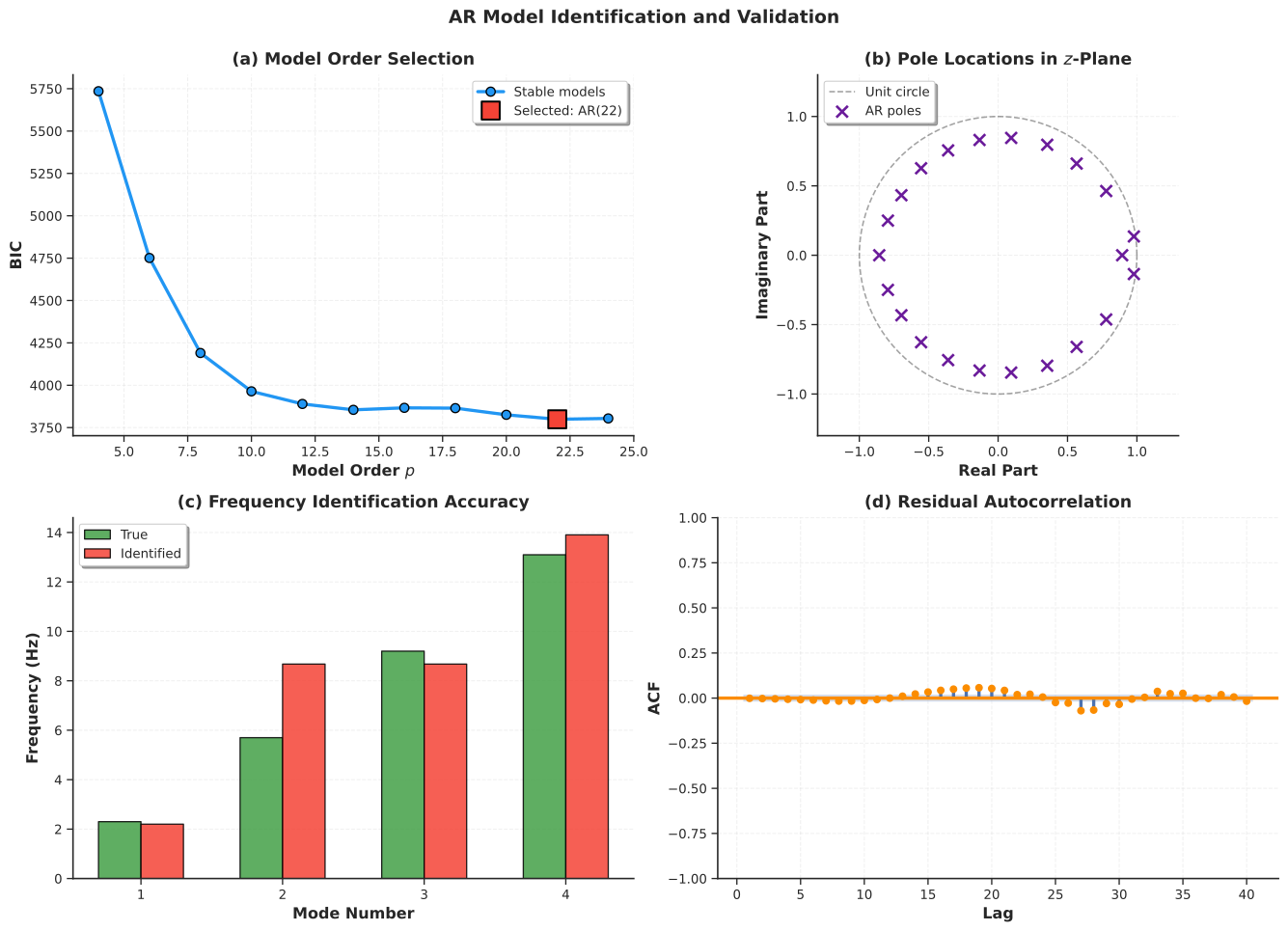
AR model identification and validation. (a) Model order selection via BIC, with the optimal order marked. (b) Pole locations in the z-plane confirming stability (all poles inside the unit circle). (c) Frequency identification accuracy comparing true and AR-identified natural frequencies. (d) Residual autocorrelation verifying whiteness of the innovation sequence. — Figure 4:AR model identification and validation. (a) Model order selection via BIC, with the optimal order marked. (b) Pole locations in the $z$ -plane confirming stability (all poles inside the unit circle). (c) Frequency identification accuracy comparing true and AR-identified natural frequencies. (d) Residual autocorrelation verifying whiteness of the innovation sequence.

4ARMA Models: Accounting for Colored Excitation¶

4.1When AR Residuals Are Not White¶

In many practical SHM scenarios, fitting an AR model to bridge acceleration data produces residuals that still show significant autocorrelation, violating the whiteness assumption. This happens because real-world excitation is rarely pure white noise. Wind gusts tend to cluster in time rather than arriving as independent impulses, traffic loads come in platoons rather than uniformly random patterns, and analog anti-aliasing filters in the data acquisition system introduce correlation into the measurement noise. When the driving excitation is colored (temporally correlated), the AR model must compensate by using an unnecessarily high order, or the residuals will carry structure that the model failed to capture.

The ARMA model addresses this limitation by adding moving average (MA) terms that explicitly model the temporal correlation in the innovation process. The AR part continues to capture the structural dynamics (poles), while the MA part captures the spectral shape of the excitation (zeros). Together, they provide a more parsimonious and accurate representation of the observed vibration when the driving forces are correlated.

ARMA models are appropriate when AR residuals show significant autocorrelation (a failed Ljung-Box test), when excitation is known to be colored (wind loading, traffic platoons), or when measurement noise is correlated due to analog filtering or sensor quantization. If an AR model already produces white residuals, the added complexity of ARMA terms is not justified.

4.2Mathematical Framework¶

ARMA( $p,q$ ) combines autoregressive dynamics with moving-average noise modeling:

x_t = \sum_{i=1}^{p} \phi_i x_{t-i} + \varepsilon_t + \sum_{j=1}^{q} \theta_j \varepsilon_{t-j}, \quad \varepsilon_t \sim \mathcal{N}(0, \sigma^2)

(7)

where $\phi_i$ are the AR coefficients (structural dynamics), $\theta_j$ are the MA coefficients (excitation correlation structure), $p$ is the AR order, and $q$ is the MA order. In operator notation this becomes $\phi(L) x_t = \theta(L) \varepsilon_t$ , where $L$ denotes the lag operator ( $L x_t = x_{t-1}$ ) and:

$\phi(L) = 1 - \phi_1 L - \phi_2 L^2 - \cdots - \phi_p L^p$ is the AR polynomial
$\theta(L) = 1 + \theta_1 L + \theta_2 L^2 + \cdots + \theta_q L^q$ is the MA polynomial

We use $L$ for the lag operator rather than $B$ (the backshift operator) to avoid notational conflict with the input matrix $\mathbf{B}$ that appears in the state-space formulation later in this chapter.

The transfer function form reveals that ARMA models produce both poles and zeros in the frequency domain:

H(z) = \frac{\theta(z^{-1})}{\phi(z^{-1})} = \frac{1 + \theta_1 z^{-1} + \cdots + \theta_q z^{-q}}{1 - \phi_1 z^{-1} - \cdots - \phi_p z^{-p}}

(8)

This provides richer spectral shaping than AR alone, because the numerator zeros can suppress or enhance particular frequency bands to match the spectral characteristics of the excitation.

4.3Stability and Invertibility¶

Two properties are required for a valid ARMA model. Stability, inherited from the AR part, requires that all roots of $\phi(z) = 0$ lie inside the unit circle ( $|\lambda_i| < 1$ ). This is the same condition as for pure AR models and ensures that the predicted response remains bounded.

Invertibility is a new requirement introduced by the MA part. It requires that all roots of $\theta(z) = 0$ lie inside the unit circle ( $|\mu_j| < 1$ ). Without invertibility, multiple distinct parameter sets $(\boldsymbol{\phi}, \boldsymbol{\theta})$ can produce identical output statistics, making the model non-identifiable. Invertibility also ensures that the innovation sequence $\varepsilon_t$ can be uniquely recovered from the observed data, which is essential for maximum likelihood estimation, Kalman filtering, and forecasting.

4.4Identification: Why ARMA Is Harder Than AR¶

AR identification is a linear problem: the Yule-Walker equations or ordinary least squares yield the coefficients directly. ARMA identification is fundamentally nonlinear because the innovation sequence $\{\varepsilon_t\}$ is latent (unobserved). To estimate the AR and MA coefficients, we need the innovations, but to compute the innovations, we need the coefficients.

The standard resolution is maximum likelihood estimation (MLE), which uses the Kalman filter internally to evaluate the likelihood function given a candidate parameter set, and then optimizes over the parameter space using gradient-based methods such as L-BFGS. The Hannan-Rissanen method provides a computationally cheaper alternative: fit a high-order AR model first to obtain approximate innovations $\hat{\varepsilon}_t$ , then regress $x_t$ on past $x$ values and past $\hat{\varepsilon}$ values to get initial ARMA estimates, and refine via Newton-Raphson. In practice, the statsmodels ARIMA implementation uses MLE with Kalman filtering and handles initialization automatically.

Model order selection proceeds by searching over a grid of $(p, q)$ candidates, fitting each combination, checking stability and invertibility, testing residual whiteness, and selecting the combination that minimizes BIC among valid models. Computational cost is roughly 5 to 10 times higher than AR due to the iterative optimization.

Algorithm 2 (ARMA Identification with Order Selection)

Input: Response time series $\{x_t\}_{t=1}^N$ , sampling frequency $f_s$ , maximum orders $p_{\max}$ , $q_{\max}$

Output: Optimal ARMA( $p^*, q^*$ ) model with stability/invertibility guarantees

Data Preprocessing:
- Remove trend: $x_t \leftarrow x_t - \text{polyfit}(t, x, \text{deg}=1)$
- Standardize: $x_t \leftarrow (x_t - \bar{x}) / \sigma_x$
- Split: Training (80%), Validation (20%)
Grid Search Loop:
- For $p = 1, 2, \ldots, p_{\max}$ :
  - For $q = 0, 1, \ldots, q_{\max}$ :
    - Fit ARMA( $p$ , $q$ ) via maximum likelihood (Kalman filter for likelihood evaluation, BFGS optimization)
    - Check stability: Roots of $\phi(z) = 0$ satisfy $|z_i| < 1$
    - Check invertibility: Roots of $\theta(z) = 0$ satisfy $|z_j| < 1$
    - Compute residuals and run Ljung-Box test
    - Compute BIC: $\text{BIC} = -2 \ln L + (p + q + 1) \ln N$
    - Store results: $(p, q, \text{BIC}, \text{stability}, \text{invertibility}, \text{LB p-value})$
Model Selection:
- Retain only models with stability = True AND invertibility = True
- Among those, prefer models with Ljung-Box $p$ -value $> 0.05$
- Select: $p^*, q^* = \arg\min_{(p,q)} \text{BIC}$ among valid models
Refit and Validate:
- Refit ARMA( $p^*$ , $q^*$ ) on full training data
- One-step-ahead prediction on validation data
- Compute NRMSE; if $> 0.3$ , consider lower $(p, q)$
Physical Plausibility:
- Extract poles from AR polynomial and convert to modal parameters
- Verify frequencies and damping ratios fall within expected ranges
Return: Fitted ARMA model, BIC grid, validation metrics

arma_identification.py

1
2
3
4
5
6
7
8
9
10
11
12
13
14
15
16
17
18
19
20
21
22
23
24
25
26
27
28
29
30
31
32
33
34
35
36
37
38
39
40
41
42
43
44
45
46
47
48
49
50
51
52
53
54
55
56
57
58
59
60
61
62
63
64
65
66
67
68
69
70
71
72
73
74
75
76
77
78
79
80
81
82
83
84
85
86
87
88
89
90
91
92
93
94
95
96
97
98
99
100
101
102
103
104
105
106
107
108
109
110
111
112
113
114
115
116
117
118
119
120
121
122
123
124
125
126
127
128
129
130
131
132
133
134
135
136
137
138
139
140
141
142
143
144
145
146
147
148
149
150
151
152
153
154
155
156
157
158
159
160
161
162
163
164
165
166
"""
ARMA Model Identification with Order Selection for Chapter 8.

Provides automated ARMA fitting via MLE grid search, residual
diagnostics, and publication-quality visualization.
"""

import numpy as np
import matplotlib.pyplot as plt
from scipy import signal, stats
from statsmodels.tsa.arima.model import ARIMA
from statsmodels.stats.diagnostic import acorr_ljungbox
from typing import Tuple
import pandas as pd
import os

from utils import (setup_plotting, COLORS, remove_spines,
                   generate_structural_response, EXAMPLE_MODES, get_output_dir)


def arma_identification(
    response: np.ndarray,
    max_p: int = 8,
    max_q: int = 4,
    ic: str = 'bic'
) -> Tuple[ARIMA, pd.DataFrame]:
    """
    Identify optimal ARMA model with automated order selection.

    Parameters
    ----------
    response : np.ndarray
        Time series data.
    max_p : int
        Maximum AR order.
    max_q : int
        Maximum MA order.
    ic : str
        Information criterion ('aic' or 'bic').

    Returns
    -------
    best_model : ARIMA
        Fitted ARMA model.
    results_df : pd.DataFrame
        Order selection grid results.
    """
    results = []
    for p in range(1, max_p + 1):
        for q in range(0, max_q + 1):
            try:
                model = ARIMA(response, order=(p, 0, q), trend='n').fit(
                    method_kwargs={'maxiter': 500, 'disp': False})
                ar_stable = True
                ma_invertible = True
                if p > 0:
                    ar_stable = np.all(np.abs(np.roots(np.r_[1, -model.arparams])) < 1.0)
                if q > 0:
                    ma_invertible = np.all(np.abs(np.roots(np.r_[1, model.maparams])) < 1.0)
                lb = acorr_ljungbox(model.resid, lags=[30], return_df=True)
                lb_pval = lb['lb_pvalue'].iloc[0]
                results.append({
                    'p': p, 'q': q, 'aic': model.aic, 'bic': model.bic,
                    'log_likelihood': model.llf, 'sigma2': np.var(model.resid),
                    'lb_pvalue': lb_pval, 'ar_stable': ar_stable,
                    'ma_invertible': ma_invertible,
                    'valid': ar_stable and ma_invertible and lb_pval > 0.05
                })
            except Exception:
                continue

    results_df = pd.DataFrame(results)
    valid = results_df[results_df['valid']]
    if len(valid) == 0:
        valid = results_df[results_df['ar_stable'] & results_df['ma_invertible']]
    if len(valid) == 0:
        raise ValueError("No valid ARMA models found")

    best_idx = valid[ic].idxmin()
    best_p = int(results_df.loc[best_idx, 'p'])
    best_q = int(results_df.loc[best_idx, 'q'])
    best_model = ARIMA(response, order=(best_p, 0, best_q), trend='n').fit(
        method_kwargs={'maxiter': 500, 'disp': False})
    return best_model, results_df


def generate_arma_figure():
    """Generate the ARMA diagnostics figure."""
    setup_plotting()
    t, acceleration = generate_structural_response(EXAMPLE_MODES, duration_s=100, fs=100)
    arma_model, arma_results = arma_identification(acceleration, max_p=6, max_q=3)

    print(f"Selected: ARMA({arma_model.model_orders['ar']}, {arma_model.model_orders['ma']})")
    print(f"BIC: {arma_model.bic:.2f}")

    fig, axes = plt.subplots(2, 2, figsize=(14, 10))

    # (a) BIC heat map
    pivot = arma_results.pivot_table(values='bic', index='p', columns='q', aggfunc='min')
    im = axes[0, 0].imshow(pivot.values, cmap='viridis_r', aspect='auto', interpolation='nearest')
    axes[0, 0].set_xticks(np.arange(len(pivot.columns)))
    axes[0, 0].set_yticks(np.arange(len(pivot.index)))
    axes[0, 0].set_xticklabels(pivot.columns)
    axes[0, 0].set_yticklabels(pivot.index)
    axes[0, 0].set_xlabel('MA Order $q$')
    axes[0, 0].set_ylabel('AR Order $p$')
    axes[0, 0].set_title('(a) BIC Heat Map', pad=8)
    bp = arma_model.model_orders['ar']
    bq = arma_model.model_orders['ma']
    bp_idx = list(pivot.index).index(bp)
    bq_idx = list(pivot.columns).index(bq)
    axes[0, 0].plot(bq_idx, bp_idx, '*', color=COLORS['warning'],
                    markersize=18, markeredgecolor='white', markeredgewidth=1.5)
    cbar = plt.colorbar(im, ax=axes[0, 0], pad=0.02, aspect=30)
    cbar.set_label('BIC', fontsize=10, fontweight='bold')

    # (b) Standardized residuals
    resid = arma_model.resid
    axes[0, 1].plot(t[:2000], resid[:2000], color=COLORS['neutral'], linewidth=0.7, alpha=0.8)
    axes[0, 1].axhline(0, color='k', linestyle='--', linewidth=1.0)
    axes[0, 1].fill_between(t[:2000], -2 * np.std(resid), 2 * np.std(resid),
                             alpha=0.15, color=COLORS['primary'])
    axes[0, 1].set_xlabel('Time (s)')
    axes[0, 1].set_ylabel('Residual')
    axes[0, 1].set_title('(b) Standardized Residuals', pad=8)
    axes[0, 1].grid(True, alpha=0.3, linestyle='--')
    remove_spines(axes[0, 1])

    # (c) Spectral whitening
    f_orig, p_orig = signal.welch(acceleration, fs=100, nperseg=2048)
    f_res, p_res = signal.welch(resid, fs=100, nperseg=1024)
    axes[1, 0].semilogy(f_orig, p_orig, color=COLORS['primary'], linewidth=2.5,
                        label='Original', alpha=0.85)
    axes[1, 0].semilogy(f_res, p_res, color=COLORS['accent'], linewidth=2.5,
                        label='ARMA residuals', linestyle='--')
    axes[1, 0].set_xlabel('Frequency (Hz)')
    axes[1, 0].set_ylabel('PSD')
    axes[1, 0].set_title('(c) Spectral Whitening', pad=8)
    axes[1, 0].set_xlim(0, 20)
    axes[1, 0].legend(loc='upper right', frameon=True, shadow=True, fontsize=10, fancybox=True)
    axes[1, 0].grid(True, alpha=0.3, linestyle='--', which='both')
    remove_spines(axes[1, 0])

    # (d) Q-Q plot
    osm, osr = stats.probplot(resid, dist="norm", fit=True)
    axes[1, 1].scatter(osm[0], osm[1], c=COLORS['teal'], s=15, alpha=0.5, edgecolors='none')
    axes[1, 1].plot(osm[0], osm[0] * osr[0] + osr[1], 'k-', linewidth=2.0, label='Normal reference')
    axes[1, 1].set_xlabel('Theoretical Quantiles')
    axes[1, 1].set_ylabel('Sample Quantiles')
    axes[1, 1].set_title('(d) Normal Q-Q Plot', pad=8)
    axes[1, 1].legend(loc='upper left', frameon=True, shadow=True, fontsize=10, fancybox=True)
    axes[1, 1].grid(True, alpha=0.3, linestyle='--')
    remove_spines(axes[1, 1])

    plt.tight_layout(rect=[0, 0, 1, 0.97])
    fig.suptitle('ARMA Model Diagnostics', fontsize=14, fontweight='bold', y=1.00)

    output_path = os.path.join(get_output_dir(), 'ch08_fig_arma_diagnostics.svg')
    plt.savefig(output_path, bbox_inches='tight')
    plt.close()
    print(f"Saved: {output_path}")
    return output_path


if __name__ == '__main__':
    generate_arma_figure()

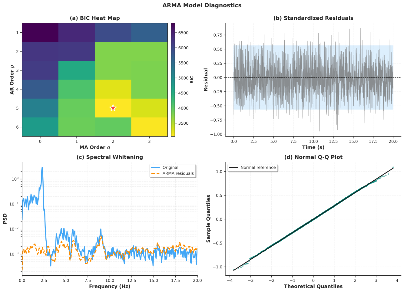
ARMA model diagnostics. (a) BIC heat map over the (p, q) order grid with the optimal model marked. (b) Standardized residuals with \pm 2\sigma bounds. (c) Spectral whitening showing the original signal PSD versus ARMA residual PSD. (d) Normal Q-Q plot verifying Gaussianity of the innovation sequence. — Figure 5:ARMA model diagnostics. (a) BIC heat map over the $(p, q)$ order grid with the optimal model marked. (b) Standardized residuals with $\pm 2\sigma$ bounds. (c) Spectral whitening showing the original signal PSD versus ARMA residual PSD. (d) Normal Q-Q plot verifying Gaussianity of the innovation sequence.

4.5Validation¶

ARMA validation follows the same principles as AR validation, with the addition of the invertibility check for the MA polynomial. The essential tests are: (1) stability of the AR polynomial, (2) invertibility of the MA polynomial, (3) residual whiteness via the Ljung-Box test, (4) comparison against the simpler AR model via the BIC difference, and (5) physical plausibility of extracted modal parameters. A BIC difference greater than 10 provides strong evidence favoring the more complex model; a difference between 2 and 10 provides moderate evidence; and a difference less than 2 suggests that the simpler AR model is adequate.

Check	Test	Pass Criteria	Action if Fail
Stability	AR roots	All $\|\lambda_i\| < 1$	Discard model
Invertibility	MA roots	All $\|\mu_j\| < 1$	Discard model
Whiteness	Ljung-Box	$p$ -value $> 0.05$	Increase $q$ or use ARMAX
Improvement	$\Delta$ BIC vs AR	$> 2$	Use AR if $< 2$
Plausibility	Modal parameters	$f \in [0.5, 50]$ Hz, $\zeta \in [0.005, 0.15]$	Check data quality

A validated ARMA model offers a meaningful advantage for damage detection, because its residuals are sensitized to structural changes while being robust to colored ambient excitation. However, an over-parameterized or poorly validated ARMA model can perform worse than a simple AR model, so validation should never be skipped.

5ARMAX Models: Incorporating Known Inputs¶

5.1When Measured Excitation Is Available¶

Consider monitoring a highway bridge with accelerometers. An ARMA model works well during stable traffic conditions, but when traffic patterns change dramatically, the residual variance increases regardless of whether the structure is damaged. The fundamental issue is that AR and ARMA models treat all excitation as unknown stochastic input. They cannot distinguish between a large response caused by heavy trucks (benign) and a large response caused by stiffness loss (damage).

The ARMAX model resolves this ambiguity by incorporating measured exogenous inputs. If the bridge is equipped with weigh-in-motion sensors that record truck weights, or strain gauges on the pavement that measure loading, these measurements can be fed into the model as known inputs $u_t$ . The model then predicts the expected response given the measured load, and the residual captures only the unexplained portion. After a healthy baseline is established, an increase in residual variance that cannot be attributed to changes in the known input is strong evidence of structural change.

ARMAX models are most valuable when reliable measurements of the excitation are available (traffic loads, wind speed, temperature), when operational variability is large relative to the damage signature, and when the primary objective is damage detection via residual monitoring. If no excitation measurements exist (the typical output-only ambient vibration scenario), AR or ARMA models are the appropriate choice.

5.2Mathematical Framework¶

The ARMAX model extends ARMA by adding exogenous input terms:

x_t = \underbrace{\sum_{i=1}^{p} \phi_i x_{t-i}}_{\text{AR: system memory}} + \underbrace{\sum_{j=0}^{r} \beta_j u_{t-j}}_{\text{Input dynamics}} + \underbrace{\varepsilon_t + \sum_{k=1}^{q} \theta_k \varepsilon_{t-k}}_{\text{MA: colored noise}}

(9)

where $u_t$ is the measured exogenous input (for example, traffic load, wind speed, or temperature), $\beta_j$ are the transfer function coefficients mapping input to output ( $j = 0, \ldots, r$ ), and $r$ is the input lag order. The remaining notation is the same as for ARMA. In compact operator form, $\phi(z) x_t = \beta(z) u_t + \theta(z) \varepsilon_t$ , where $\beta(z) = \beta_0 + \beta_1 z^{-1} + \cdots + \beta_r z^{-r}$ .

The input-to-output transfer function is:

H(z) = \frac{\beta(z)}{\phi(z)} = \frac{\sum_{j=0}^{r} \beta_j z^{-j}}{1 - \sum_{i=1}^{p} \phi_i z^{-i}}

(10)

This is the discrete-time frequency response function (FRF). Its poles are the same as those of the AR polynomial and yield the modal parameters $(f_n, \zeta)$ , while the numerator coefficients $\beta_j$ encode the sensor and actuator placement geometry and mode shapes. The full response can be decomposed as $x_t = H(z) u_t + G(z) \varepsilon_t$ , separating the deterministic part (from known input) and the stochastic part (from unknown excitation).

Progressive hierarchy of parametric time-series models from AR(p) through ARMA(p, q) and ARMAX(p, q, r) to the state-space representation \mathbf{x}_{t+1} = \mathbf{A}\mathbf{x}_t + \mathbf{B}\mathbf{u}_t,\ \mathbf{y}_t = \mathbf{C}\mathbf{x}_t + \mathbf{D}\mathbf{u}_t. Each level adds modelling capability: MA terms \sum \theta_j \varepsilon_{t-j} capture coloured noise, exogenous inputs \sum \beta_k u_{t-k} account for known excitation, and the matrix formulation enables MIMO systems and optimal Kalman filtering. 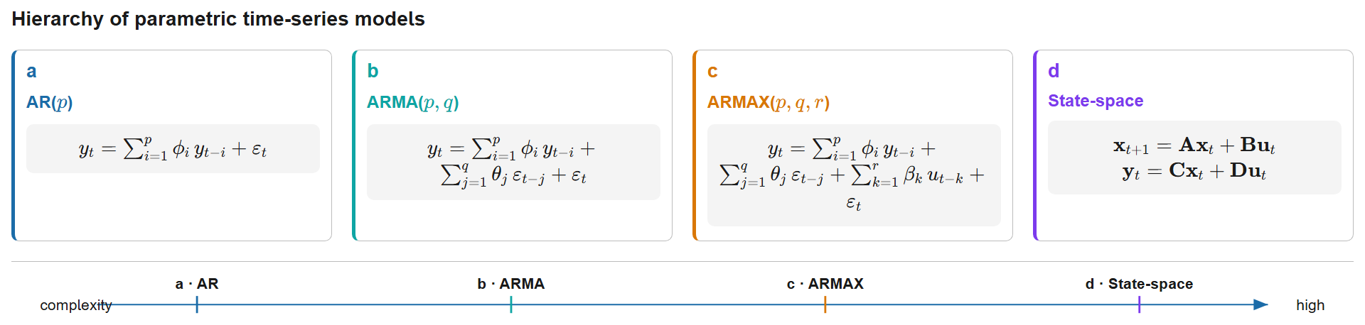— Figure 6:Progressive hierarchy of parametric time-series models from AR( $p$ ) through ARMA( $p, q$ ) and ARMAX( $p, q, r$ ) to the state-space representation $\mathbf{x}_{t+1} = \mathbf{A}\mathbf{x}_t + \mathbf{B}\mathbf{u}_t,\ \mathbf{y}_t = \mathbf{C}\mathbf{x}_t + \mathbf{D}\mathbf{u}_t$ . Each level adds modelling capability: MA terms $\sum \theta_j \varepsilon_{t-j}$ capture coloured noise, exogenous inputs $\sum \beta_k u_{t-k}$ account for known excitation, and the matrix formulation enables MIMO systems and optimal Kalman filtering.

5.3Validity Requirements¶

Three properties are required for a physically meaningful ARMAX model. Stability and invertibility carry the same meaning as in ARMA. Causality is a new requirement specific to ARMAX: the input lag order must satisfy $r \leq p$ , because the response at time $t$ cannot depend on future inputs. Violation of this constraint implies a non-causal model, which is physically meaningless.

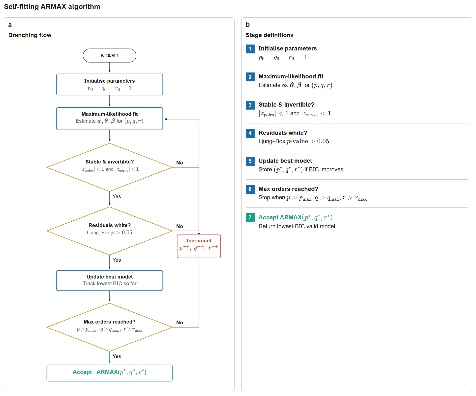
Automated ARMAX(p, q, r) order-selection workflow with integrated validation. The algorithm iteratively fits candidate models by maximum likelihood, enforces stability (|z_{\text{poles}}| < 1) and invertibility (|z_{\text{zeros}}| < 1), validates residual whiteness via the Ljung-Box test (p > 0.05), and selects optimal orders by tracking the minimum BIC over all combinations. — Figure 7:Automated ARMAX( $p, q, r$ ) order-selection workflow with integrated validation. The algorithm iteratively fits candidate models by maximum likelihood, enforces stability ( $|z_{\text{poles}}| < 1$ ) and invertibility ( $|z_{\text{zeros}}| < 1$ ), validates residual whiteness via the Ljung-Box test ( $p > 0.05$ ), and selects optimal orders by tracking the minimum BIC over all combinations.

Algorithm 3 (ARMAX Identification with Exogenous Inputs)

Input: Response $\{x_t\}_{t=1}^N$ , exogenous input $\{u_t\}_{t=1}^N$ , sampling frequency $f_s$ , order candidates $(p_{\max}, q_{\max}, r_{\max})$

Output: Optimal ARMAX( $p^*, q^*, r^*$ ) model with damage detection capability

Data Preprocessing:
- Synchronize $x_t$ and $u_t$ (verify via cross-correlation; even 1-sample misalignment corrupts the transfer function)
- Remove trends from both signals
- Standardize both signals to zero mean and unit variance
- Split: Training (70%), Validation (30%)
Grid Search Loop:
- For $p = 2, \ldots, p_{\max}$ ; $q = 0, \ldots, q_{\max}$ ; $r = 0, \ldots, \min(r_{\max}, p)$ (enforcing causality $r \leq p$ ):
  - Fit ARMAX( $p$ , $q$ , $r$ ) via MLE using SARIMAX with exogenous input matrix
  - Check stability (AR roots inside unit circle), invertibility (MA roots inside unit circle)
  - Compute residuals and Ljung-Box $p$ -value
  - Compute BIC: $\text{BIC} = -2 \ln L + (p + q + r + 1) \ln N$
Model Selection:
- Retain models satisfying stability, invertibility, and causality
- Among those, select $(p^*, q^*, r^*) = \arg\min \text{BIC}$
Validation:
- One-step-ahead prediction on hold-out data; compute NRMSE (accept if $< 0.25$ )
- Extract transfer function $H(z)$ and verify resonance peaks match expected modal frequencies
- Verify residual whiteness with Ljung-Box $p$ -value $> 0.05$
Baseline Storage:
- Save fitted parameters, residual statistics (mean, variance, distribution)
- This becomes the healthy-structure reference for online damage detection
Return: Fitted ARMAX model, transfer function $H(z)$ , BIC grid, validation metrics, baseline residuals

5.4Application: Damage Detection via Residual Variance¶

When structural damage occurs (stiffness reduction, connection loosening), the system transfer function changes. An ARMAX model fitted to the healthy baseline can no longer accurately predict the damaged response, even when accounting for the known input. This manifests as three measurable signatures: increased residual variance (the model’s predictions become less accurate), changed transfer function coefficients (the pole locations shift, reflecting altered modal parameters), and violation of residual whiteness (the model can no longer explain the temporal structure of the response).

The damage detection strategy is straightforward. During baseline monitoring, fit an ARMAX model on data from the healthy structure and record the residual variance $\sigma_{\text{healthy}}^2$ . During online monitoring, use the baseline model to predict new measurements given the current input, compute the residual variance $\sigma_{\text{new}}^2$ , and form the variance ratio $\sigma_{\text{new}}^2 / \sigma_{\text{healthy}}^2$ . A ratio significantly exceeding 1.0 (typically above 1.5) indicates that the structure has changed in a way that the baseline model cannot explain via known operational inputs alone.

The key advantage of ARMAX over AR or ARMA for damage detection is that the exogenous input $u_t$ accounts for operational variability. When traffic increases, both the response and the input increase together, so the ARMAX residual remains small. But when stiffness decreases, the response changes in a way that the input alone cannot explain, causing the residual to grow.

armax_damage_detection.py

1
2
3
4
5
6
7
8
9
10
11
12
13
14
15
16
17
18
19
20
21
22
23
24
25
26
27
28
29
30
31
32
33
34
35
36
37
38
39
40
41
42
43
44
45
46
47
48
49
50
51
52
53
54
55
56
57
58
59
60
61
62
63
64
65
66
67
68
69
70
71
72
73
74
75
76
77
78
79
80
81
82
83
84
85
86
87
88
89
90
91
92
93
94
95
96
97
98
99
100
101
102
103
104
105
106
107
108
109
110
111
112
113
114
115
116
117
118
119
120
121
122
123
124
125
126
127
128
129
130
131
132
133
134
135
136
137
138
139
140
141
142
143
144
145
146
147
148
149
150
151
152
153
154
155
156
157
158
159
160
161
162
163
164
165
166
167
168
169
170
171
172
173
174
175
176
177
178
179
180
"""
ARMAX Damage Detection for Chapter 8.

Simulates healthy and damaged structural responses to known excitation,
fits an ARMAX baseline model, and visualizes residual-based damage detection.
"""

import numpy as np
import matplotlib.pyplot as plt
from scipy import signal, stats
from statsmodels.tsa.statespace.sarimax import SARIMAX
from typing import Tuple
import os

from utils import setup_plotting, COLORS, remove_spines, get_output_dir


def simulate_damage_scenario(
    baseline_frequency: float = 4.5,
    baseline_damping: float = 0.02,
    damage_frequency_shift: float = -0.15,
    damage_damping_increase: float = 0.002,
    duration_s: float = 120,
    fs: float = 50,
    seed: int = 100
) -> Tuple[np.ndarray, np.ndarray, np.ndarray, np.ndarray]:
    """
    Simulate healthy and damaged responses to known excitation.

    Returns
    -------
    t, excitation, response_healthy, response_damaged
    """
    rng = np.random.default_rng(seed)
    dt = 1 / fs
    t = np.arange(0, duration_s, dt)
    n = len(t)

    background = signal.lfilter([1], [1, -0.7], rng.standard_normal(n))
    n_vehicles = rng.poisson(lam=20)
    crossing_times = rng.choice(n, size=n_vehicles, replace=False)
    impulses = np.zeros(n)
    impulses[crossing_times] = rng.uniform(1.5, 4.0, size=n_vehicles)
    excitation = 0.5 * background + signal.lfilter([1], [1, -0.4], impulses)

    # Healthy system
    wn_h = 2 * np.pi * baseline_frequency
    num_h, den_h = [wn_h**2], [1, 2 * baseline_damping * wn_h, wn_h**2]
    num_h_d, den_h_d, _ = signal.cont2discrete((num_h, den_h), dt)
    response_healthy = signal.lfilter(num_h_d.flatten(), den_h_d.flatten(), excitation)
    response_healthy += 0.03 * np.std(response_healthy) * rng.standard_normal(n)

    # Damaged system
    wn_d = 2 * np.pi * (baseline_frequency + damage_frequency_shift)
    zeta_d = baseline_damping + damage_damping_increase
    num_d, den_d = [wn_d**2], [1, 2 * zeta_d * wn_d, wn_d**2]
    num_d_d, den_d_d, _ = signal.cont2discrete((num_d, den_d), dt)
    response_damaged = signal.lfilter(num_d_d.flatten(), den_d_d.flatten(), excitation)
    response_damaged += 0.03 * np.std(response_damaged) * rng.standard_normal(n)

    return t, excitation, response_healthy, response_damaged


def fit_armax(output, exog_input, p=3, q=1, r=2):
    """Fit ARMAX model with lagged inputs."""
    exog = np.column_stack([np.roll(exog_input, i) for i in range(r + 1)])
    start = max(p, q, r)
    model = SARIMAX(output[start:], order=(p, 0, q), exog=exog[start:], trend='n').fit(
        disp=False, maxiter=200)
    return model


def compute_armax_residuals(model, output, exog_input, r=2):
    """Compute prediction residuals using baseline model."""
    exog = np.column_stack([np.roll(exog_input, i) for i in range(r + 1)])
    p, q = model.model_orders['ar'], model.model_orders['ma']
    start = max(p, q, r)
    predictions = model.predict(start=0, end=len(output[start:]) - 1, exog=exog[start:])
    return output[start:] - predictions


def generate_armax_figure():
    """Generate the ARMAX damage detection figure."""
    setup_plotting()

    t_dmg, load, resp_healthy, resp_damaged = simulate_damage_scenario()
    baseline_model = fit_armax(resp_healthy, load, p=3, q=1, r=2)

    resid_healthy = compute_armax_residuals(baseline_model, resp_healthy, load)
    resid_damaged = compute_armax_residuals(baseline_model, resp_damaged, load)

    variance_ratio = np.var(resid_damaged) / np.var(resid_healthy)
    print(f"Variance ratio (damaged/healthy): {variance_ratio:.3f}")
    print(f"Interpretation: {100*(variance_ratio-1):.1f}% increase")

    fig, axes = plt.subplots(3, 2, figsize=(14, 12))

    # (a) Input signal
    axes[0, 0].plot(t_dmg[:1000], load[:1000], color=COLORS['neutral'], linewidth=1.2)
    axes[0, 0].set_xlabel('Time (s)')
    axes[0, 0].set_ylabel('Load Amplitude')
    axes[0, 0].set_title('(a) Measured Excitation Input', pad=8)
    axes[0, 0].grid(True, alpha=0.3, linestyle='--')
    remove_spines(axes[0, 0])

    # (b) Healthy vs damaged response
    axes[0, 1].plot(t_dmg[:1000], resp_healthy[:1000], color=COLORS['success'],
                    linewidth=1.5, label='Healthy', alpha=0.85)
    axes[0, 1].plot(t_dmg[:1000], resp_damaged[:1000], color=COLORS['warning'],
                    linewidth=1.2, label='Damaged', alpha=0.75)
    axes[0, 1].set_xlabel('Time (s)')
    axes[0, 1].set_ylabel('Response')
    axes[0, 1].set_title('(b) Structural Response', pad=8)
    axes[0, 1].legend(loc='upper right', frameon=True, shadow=True, fontsize=10, fancybox=True)
    axes[0, 1].grid(True, alpha=0.3, linestyle='--')
    remove_spines(axes[0, 1])

    # (c) Healthy residuals
    t_resid = t_dmg[3:][:len(resid_healthy)]
    axes[1, 0].plot(t_resid[:800], resid_healthy[:800], color=COLORS['success'],
                    linewidth=0.9, alpha=0.75)
    axes[1, 0].axhline(0, color='k', linestyle='--', linewidth=1.0)
    axes[1, 0].fill_between(t_resid[:800], -2 * np.std(resid_healthy),
                             2 * np.std(resid_healthy), alpha=0.12, color=COLORS['success'])
    axes[1, 0].set_xlabel('Time (s)')
    axes[1, 0].set_ylabel('Residual')
    axes[1, 0].set_title('(c) Healthy Baseline Residuals', pad=8)
    axes[1, 0].grid(True, alpha=0.3, linestyle='--')
    remove_spines(axes[1, 0])

    # (d) Damaged residuals
    axes[1, 1].plot(t_resid[:800], resid_damaged[:800], color=COLORS['warning'],
                    linewidth=0.9, alpha=0.75)
    axes[1, 1].axhline(0, color='k', linestyle='--', linewidth=1.0)
    axes[1, 1].fill_between(t_resid[:800], -2 * np.std(resid_damaged),
                             2 * np.std(resid_damaged), alpha=0.12, color=COLORS['warning'])
    axes[1, 1].set_xlabel('Time (s)')
    axes[1, 1].set_ylabel('Residual')
    axes[1, 1].set_title('(d) Damaged Structure Residuals', pad=8)
    axes[1, 1].grid(True, alpha=0.3, linestyle='--')
    remove_spines(axes[1, 1])

    # (e) Healthy distribution
    axes[2, 0].hist(resid_healthy, bins=45, density=True, color=COLORS['success'],
                    alpha=0.7, edgecolor='black', linewidth=0.5)
    axes[2, 0].axvline(0, color='k', linestyle='--', linewidth=1.0)
    axes[2, 0].set_xlabel('Residual Value')
    axes[2, 0].set_ylabel('Density')
    axes[2, 0].set_title('(e) Healthy Residual Distribution', pad=8)
    axes[2, 0].grid(True, alpha=0.3, linestyle='--', axis='y')
    remove_spines(axes[2, 0])

    # (f) Damaged distribution
    axes[2, 1].hist(resid_damaged, bins=45, density=True, color=COLORS['warning'],
                    alpha=0.7, edgecolor='black', linewidth=0.5)
    axes[2, 1].axvline(0, color='k', linestyle='--', linewidth=1.0)
    axes[2, 1].text(0.97, 0.95, f'Variance ratio = {variance_ratio:.2f}',
                    transform=axes[2, 1].transAxes, fontsize=10, fontweight='bold',
                    ha='right', va='top',
                    bbox=dict(boxstyle='round,pad=0.4', facecolor=COLORS['light_red'],
                              edgecolor=COLORS['dark_red'], linewidth=1.5))
    axes[2, 1].set_xlabel('Residual Value')
    axes[2, 1].set_ylabel('Density')
    axes[2, 1].set_title('(f) Damaged Residual Distribution', pad=8)
    axes[2, 1].grid(True, alpha=0.3, linestyle='--', axis='y')
    remove_spines(axes[2, 1])

    plt.tight_layout(rect=[0, 0, 1, 0.97])
    fig.suptitle('ARMAX-Based Damage Detection: Residual Analysis',
                 fontsize=14, fontweight='bold', y=1.00)

    output_path = os.path.join(get_output_dir(), 'ch08_fig_armax_damage.svg')
    plt.savefig(output_path, bbox_inches='tight')
    plt.close()
    print(f"Saved: {output_path}")
    return output_path


if __name__ == '__main__':
    generate_armax_figure()

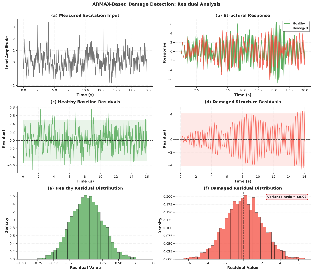
$ARMAX-based damage detection: residual analysis. (a) Measured excitation input (traffic-like loading). (b) Structural response comparison between healthy and damaged conditions. (c) Healthy baseline residuals within \pm 2\sigma bounds. (d) Damaged structure residuals showing increased variance. (e) Healthy residual distribution. (f) Damaged residual distribution with annotated variance ratio indicating structural change.$

Figure 8:ARMAX-based damage detection: residual analysis. (a) Measured excitation input (traffic-like loading). (b) Structural response comparison between healthy and damaged conditions. (c) Healthy baseline residuals within $\pm 2\sigma$ bounds. (d) Damaged structure residuals showing increased variance. (e) Healthy residual distribution. (f) Damaged residual distribution with annotated variance ratio indicating structural change.

5.5Validation Summary¶

ARMAX validation includes all the checks from ARMA plus three additional requirements unique to the input-output setting. Input-output synchronization should be verified using cross-correlation; even a one-sample misalignment between $x_t$ and $u_t$ corrupts the estimated transfer function. Causality ( $r \leq p$ ) must hold. The transfer function should be physically plausible, with resonance peaks matching known modal frequencies.

Check	Test	Pass Criteria	Action if Fail
Synchronization	Cross-correlation	Lag $\leq$ 1 sample	Re-align time series
Stability	AR roots	All $\|\lambda_i\| < 1$	Discard model
Invertibility	MA roots	All $\|\mu_j\| < 1$	Discard model
Causality	Input lags	$r \leq p$	Reduce $r$ or increase $p$
Whiteness	Ljung-Box	$p$ -value $> 0.05$	Increase $q$ or $r$
FRF plausibility	Resonance peaks	Match known modes	Check data quality
Cross-validation	NRMSE	$< 0.30$	Simplify model

6State-Space Representation¶

6.1From Single-Channel Models to Multi-Sensor Fusion¶

The AR, ARMA, and ARMAX models developed so far treat vibration as a scalar time series from a single sensor channel. Real SHM systems, however, involve arrays of accelerometers, strain gauges, displacement sensors, and GPS receivers distributed across a structure. State-space models provide the mathematical framework for multi-sensor fusion by explicitly representing the internal states of the structure (displacements, velocities, modal coordinates) and relating them to all sensor measurements simultaneously.

State-space models also bridge the gap between data-driven time-series methods and physics-based structural dynamics. The state-space matrices are constructed directly from the mass, damping, and stiffness matrices of the equation of motion, so every matrix element has a clear physical meaning. This makes state-space the natural representation for optimal state estimation via the Kalman filter, which is the subject of the following section.

6.2Continuous-Time Formulation¶

For a structural system governed by the second-order equation of motion:

\mathbf{M}\ddot{\mathbf{x}}(t) + \mathbf{C}\dot{\mathbf{x}}(t) + \mathbf{K}\mathbf{x}(t) = \mathbf{f}(t)

(11)

where $\mathbf{x}(t) \in \mathbb{R}^n$ is the displacement vector, $\mathbf{M}$ , $\mathbf{C}$ , $\mathbf{K} \in \mathbb{R}^{n \times n}$ are the mass, damping, and stiffness matrices, and $\mathbf{f}(t) \in \mathbb{R}^n$ is the external force vector.

Defining the state vector $\mathbf{z}(t) \in \mathbb{R}^{2n}$ as the concatenation of displacements and velocities:

\mathbf{z}(t) = \begin{bmatrix} \mathbf{x}(t) \\ \dot{\mathbf{x}}(t) \end{bmatrix}

(12)

the equation of motion becomes a first-order system:

\begin{aligned} \dot{\mathbf{z}}(t) &= \mathbf{A}_c \mathbf{z}(t) + \mathbf{B}_c \mathbf{u}(t) \\ \mathbf{y}(t) &= \mathbf{H}_c \mathbf{z}(t) + \mathbf{D}_c \mathbf{u}(t) \end{aligned}

(13)

where the state-space matrices are:

\mathbf{A}_c = \begin{bmatrix} \mathbf{0}_{n \times n} & \mathbf{I}_{n \times n} \\ -\mathbf{M}^{-1}\mathbf{K} & -\mathbf{M}^{-1}\mathbf{C} \end{bmatrix} \in \mathbb{R}^{2n \times 2n}, \quad \mathbf{B}_c = \begin{bmatrix} \mathbf{0}_{n \times n} \\ \mathbf{M}^{-1} \end{bmatrix} \in \mathbb{R}^{2n \times n}

(14)

The matrix $\mathbf{A}_c$ is the state transition matrix governing free vibration dynamics. Its upper-right block ( $\mathbf{I}$ ) simply expresses the kinematic relation $\dot{x} = v$ ; its lower-left block ( $-\mathbf{M}^{-1}\mathbf{K}$ ) represents the restoring forces; and its lower-right block ( $-\mathbf{M}^{-1}\mathbf{C}$ ) represents the dissipative forces. The matrix $\mathbf{B}_c$ maps external forces to state derivatives. The matrix $\mathbf{H}_c$ is the measurement matrix that maps states to sensor outputs (for example, extracting accelerations at instrumented locations). We use $\mathbf{H}$ rather than $\mathbf{C}$ for the measurement matrix to avoid notational conflict with the damping matrix. The matrix $\mathbf{D}_c$ is the direct feedthrough matrix, which is typically zero for structural systems because the response is not instantaneous.

For structures with well-separated modes, modal decomposition provides an efficient state-space formulation. Transforming to modal coordinates via $\mathbf{x}(t) = \boldsymbol{\Phi} \mathbf{q}(t)$ , where $\boldsymbol{\Phi}$ is the mode shape matrix and $\mathbf{q}(t)$ are the modal amplitudes, decouples the system into independent oscillators. Each mode satisfies $\ddot{q}_i + 2\zeta_i \omega_{n,i} \dot{q}_i + \omega_{n,i}^2 q_i = f_i(t)$ , which in state-space form with $\mathbf{z}_i = [q_i, \dot{q}_i]^\top$ becomes:

For $m$ modes, the global state-space matrices are assembled in block-diagonal form: $\mathbf{A}_c = \text{blkdiag}(\mathbf{A}_{c,1}, \ldots, \mathbf{A}_{c,m}) \in \mathbb{R}^{2m \times 2m}$ . This structure is computationally efficient and reveals which modes dominate the response.

6.4Discrete-Time Transformation¶

Digital sensors sample at discrete times $t_k = k\Delta t$ , so the continuous-time model must be discretized. The exact discrete-time equivalent, assuming zero-order hold on inputs, is:

\begin{aligned} \mathbf{z}_{k+1} &= \mathbf{A}_d \mathbf{z}_k + \mathbf{B}_d \mathbf{u}_k + \mathbf{w}_k \\ \mathbf{y}_k &= \mathbf{H}_d \mathbf{z}_k + \mathbf{v}_k \end{aligned}

(16)

where $\mathbf{w}_k \sim \mathcal{N}(\mathbf{0}, \mathbf{Q})$ is process noise (modeling uncertainties and unmeasured disturbances) and $\mathbf{v}_k \sim \mathcal{N}(\mathbf{0}, \mathbf{R})$ is measurement noise (sensor inaccuracies). The discrete matrices are obtained via matrix exponential:

\mathbf{A}_d = e^{\mathbf{A}_c \Delta t}, \quad \mathbf{B}_d = \mathbf{A}_c^{-1}(\mathbf{A}_d - \mathbf{I})\mathbf{B}_c

(17)

The matrix exponential provides exact discretization for linear systems, preserving stability properties and eigenvalue relationships. This is important because the first-order Euler approximation $\mathbf{A}_d \approx \mathbf{I} + \mathbf{A}_c \Delta t$ can introduce significant errors for fast dynamics or low sampling rates.

6.5Observability¶

A fundamental question in sensor-based monitoring is whether the chosen sensor configuration can uniquely determine all modal states. The answer depends on the observability of the discrete-time system, which is determined by the rank of the observability matrix:

\mathcal{O} = \begin{bmatrix} \mathbf{H}_d \\ \mathbf{H}_d \mathbf{A}_d \\ \mathbf{H}_d \mathbf{A}_d^2 \\ \vdots \\ \mathbf{H}_d \mathbf{A}_d^{n-1} \end{bmatrix} \in \mathbb{R}^{np \times n}

(18)

The system is observable if and only if $\text{rank}(\mathcal{O}) = n$ (full column rank). Physically, a mode is unobservable when its mode shape has zero amplitude at all sensor locations. For example, placing accelerometers only along the nodal line of a torsional mode makes that mode invisible. Unobservable modes cannot be reconstructed by any filtering algorithm, which is why optimal sensor placement (Chapter 6) is an essential prerequisite for state-space-based monitoring.

Algorithm 4 (State-Space Model Construction from Modal Parameters)

Input: Modal frequencies $\{\omega_{n,i}\}_{i=1}^m$ , damping ratios $\{\zeta_i\}_{i=1}^m$ , sampling interval $\Delta t$

Output: Discrete state-space matrices $(\mathbf{A}_d, \mathbf{B}_d, \mathbf{H}_d)$

Build continuous-time modal matrices:
- For each mode $i = 1, \ldots, m$ :
  $\mathbf{A}_{c,i} = \begin{bmatrix} 0 & 1 \\ -\omega_{n,i}^2 & -2\zeta_i\omega_{n,i} \end{bmatrix}, \quad \mathbf{B}_{c,i} = \begin{bmatrix} 0 \\ 1 \end{bmatrix}, \quad \mathbf{H}_{c,i} = \begin{bmatrix} 1 & 0 \end{bmatrix}$
  (19)
- Assemble block-diagonal: $\mathbf{A}_c = \text{blkdiag}(\mathbf{A}_{c,1}, \ldots, \mathbf{A}_{c,m})$
Discretize via matrix exponential:
- Compute $\mathbf{A}_d = \exp(\mathbf{A}_c \Delta t)$ using scipy.linalg.expm
- If $\mathbf{A}_c$ is invertible: $\mathbf{B}_d = \mathbf{A}_c^{-1}(\mathbf{A}_d - \mathbf{I})\mathbf{B}_c$
- Otherwise: $\mathbf{B}_d = \mathbf{B}_c \Delta t$
- Set $\mathbf{H}_d = \mathbf{H}_c$ (measurement matrix unchanged)
Verify stability:
- Compute eigenvalues $\lambda_i$ of $\mathbf{A}_d$
- Check $|\lambda_i| < 1$ for all $i$ (discrete-time stability)
- If unstable, reduce $\Delta t$ or check modal parameters

state_space_model.py

1
2
3
4
5
6
7
8
9
10
11
12
13
14
15
16
17
18
19
20
21
22
23
24
25
26
27
28
29
30
31
32
33
34
35
36
37
38
39
40
41
42
43
44
45
46
47
48
49
50
51
52
53
54
55
56
57
58
59
60
61
62
63
64
65
66
67
68
69
70
71
72
73
74
75
76
77
78
79
80
81
82
83
84
85
86
87
88
89
90
91
92
93
94
95
96
97
98
99
100
101
102
103
104
105
106
107
108
109
110
111
112
113
114
115
116
117
118
119
120
121
122
123
124
125
126
127
128
129
130
131
132
133
134
135
136
137
138
139
140
141
142
143
144
145
146
147
148
149
150
151
152
153
154
155
156
157
158
159
160
161
162
163
164
165
166
167
168
169
170
171
172
173
174
175
176
177
178
179
180
181
182
183
184
185
186
187
188
"""
State-Space Model Construction and Simulation for Chapter 8.

Provides the ModalStateSpaceModel class for building, discretizing,
simulating, and visualizing modal state-space models.
"""

import numpy as np
import matplotlib.pyplot as plt
from scipy import signal, linalg
from typing import Tuple, Optional
import os

from utils import (setup_plotting, COLORS, remove_spines,
                   StructuralMode, get_output_dir)


class ModalStateSpaceModel:
    """State-space model in modal coordinates for structural dynamics."""

    def __init__(self, frequencies_hz, damping_ratios, mode_shapes=None):
        self.frequencies_hz = np.asarray(frequencies_hz)
        self.damping_ratios = np.asarray(damping_ratios)
        self.n_modes = len(frequencies_hz)
        self.mode_shapes = mode_shapes
        self.omega_n = 2 * np.pi * self.frequencies_hz
        self.omega_d = self.omega_n * np.sqrt(1 - self.damping_ratios**2)
        self._build_continuous_ss()

    def _build_continuous_ss(self):
        n = 2 * self.n_modes
        self.A_c = np.zeros((n, n))
        self.B_c = np.zeros((n, self.n_modes))
        self.H_c = np.zeros((self.n_modes, n))
        self.D_c = np.zeros((self.n_modes, self.n_modes))
        for i in range(self.n_modes):
            idx = 2 * i
            wn, zeta = self.omega_n[i], self.damping_ratios[i]
            self.A_c[idx:idx+2, idx:idx+2] = [[0, 1], [-wn**2, -2 * zeta * wn]]
            self.B_c[idx + 1, i] = 1.0
            self.H_c[i, idx] = 1.0

    def discretize(self, dt):
        self.dt, self.fs = dt, 1 / dt
        self.A_d = linalg.expm(self.A_c * dt)
        n = self.A_c.shape[0]
        if np.linalg.matrix_rank(self.A_c) == n:
            self.B_d = linalg.solve(self.A_c, (self.A_d - np.eye(n))) @ self.B_c
        else:
            self.B_d = self.B_c * dt
        self.H_d = self.H_c.copy()
        self.D_d = self.D_c.copy()
        return self

    def simulate(self, input_signal, z0=None, process_noise_std=0.0,
                 measurement_noise_std=0.0, seed=42):
        if not hasattr(self, 'A_d'):
            raise ValueError("Call .discretize(dt) first.")
        rng = np.random.default_rng(seed)
        if input_signal.ndim == 1:
            input_signal = input_signal.reshape(-1, 1)
        n_steps, n_states = input_signal.shape[0], self.A_d.shape[0]
        states = np.zeros((n_steps, n_states))
        outputs = np.zeros((n_steps, self.n_modes))
        if z0 is not None:
            states[0] = z0
        for k in range(n_steps - 1):
            w = rng.normal(0, process_noise_std, n_states)
            states[k+1] = self.A_d @ states[k] + self.B_d @ input_signal[k] + w
            v = rng.normal(0, measurement_noise_std, self.n_modes)
            outputs[k+1] = self.H_d @ states[k+1] + v
        return states, outputs

    def get_frequency_response(self, frequencies_hz):
        omega = 2 * np.pi * frequencies_hz
        n = self.A_c.shape[0]
        H = np.zeros((len(omega), self.n_modes, self.n_modes), dtype=complex)
        for i, w in enumerate(omega):
            H[i] = self.H_c @ linalg.inv(1j * w * np.eye(n) - self.A_c) @ self.B_c + self.D_c
        return H

    def check_observability(self):
        n = self.A_d.shape[0]
        O = self.H_d.copy()
        Ap = self.A_d.copy()
        for _ in range(1, n):
            O = np.vstack([O, self.H_d @ Ap])
            Ap = Ap @ self.A_d
        rank = np.linalg.matrix_rank(O)
        return (rank == n), rank


def generate_statespace_figure():
    """Generate the state-space model properties figure."""
    setup_plotting()

    bridge_modes = [
        StructuralMode(frequency_hz=2.8, damping_ratio=0.02),
        StructuralMode(frequency_hz=6.2, damping_ratio=0.025),
        StructuralMode(frequency_hz=10.5, damping_ratio=0.03),
    ]
    ss = ModalStateSpaceModel(
        frequencies_hz=np.array([m.frequency_hz for m in bridge_modes]),
        damping_ratios=np.array([m.damping_ratio for m in bridge_modes])
    ).discretize(dt=0.01)

    rng = np.random.default_rng(200)
    n_samples = 6000
    exc = signal.lfilter([1], [1, -0.75], rng.standard_normal((n_samples, 3)))
    states, measurements = ss.simulate(exc, process_noise_std=1e-4, measurement_noise_std=5e-3)
    is_obs, rank_obs = ss.check_observability()

    print(f"State dim: {ss.A_d.shape[0]}, Observable: {is_obs} (rank {rank_obs})")
    eig_d = linalg.eigvals(ss.A_d)
    print(f"Stable: {np.all(np.abs(eig_d) < 1.0)}")

    fig = plt.figure(figsize=(14, 12))
    gs = fig.add_gridspec(3, 2, hspace=0.35, wspace=0.3)
    mode_colors = [COLORS['primary'], COLORS['accent'], COLORS['teal']]

    # (a) Poles
    ax1 = fig.add_subplot(gs[0, 0])
    th = np.linspace(0, 2 * np.pi, 200)
    ax1.plot(np.cos(th), np.sin(th), 'k--', linewidth=1.2, alpha=0.4, label='Unit circle')
    ax1.scatter(eig_d.real, eig_d.imag, marker='x', c=COLORS['secondary'],
                s=100, linewidths=2.5, zorder=5, label='Discrete poles')
    ax1.set_xlabel('Real Part')
    ax1.set_ylabel('Imaginary Part')
    ax1.set_title('(a) Discrete-Time Poles', pad=8)
    ax1.set_aspect('equal')
    ax1.grid(True, alpha=0.3, linestyle='--')
    ax1.legend(loc='upper left', frameon=True, shadow=True, fontsize=9, fancybox=True)
    ax1.set_xlim(-1.3, 1.3); ax1.set_ylim(-0.1, 1.3)
    remove_spines(ax1)

    # (b) Frequency response
    ax2 = fig.add_subplot(gs[0, 1])
    freq_eval = np.logspace(-0.5, 1.5, 300)
    H_frf = ss.get_frequency_response(freq_eval)
    for i in range(3):
        mag = 20 * np.log10(np.abs(H_frf[:, i, i]) + 1e-10)
        ax2.semilogx(freq_eval, mag, linewidth=2.5, color=mode_colors[i], label=f'Mode {i+1}')
    for f in ss.frequencies_hz:
        ax2.axvline(f, color=COLORS['neutral'], linestyle=':', alpha=0.5)
    ax2.set_xlabel('Frequency (Hz)')
    ax2.set_ylabel('Magnitude (dB)')
    ax2.set_title('(b) Frequency Response $H(j\\omega)$', pad=8)
    ax2.grid(True, alpha=0.3, linestyle='--', which='both')
    ax2.legend(loc='upper right', frameon=True, shadow=True, fontsize=9, fancybox=True)
    remove_spines(ax2)

    # (c) Modal displacements
    ax3 = fig.add_subplot(gs[1, :])
    t_sim = np.arange(n_samples) * ss.dt
    for i in range(3):
        ax3.plot(t_sim[:1500], states[:1500, 2*i], linewidth=1.5,
                 label=f'Mode {i+1}', alpha=0.85, color=mode_colors[i])
    ax3.set_xlabel('Time (s)')
    ax3.set_ylabel('Modal Displacement $q(t)$')
    ax3.set_title('(c) State Vector Evolution', pad=8)
    ax3.legend(loc='upper right', frameon=True, shadow=True, fontsize=9, fancybox=True, ncol=3)
    ax3.grid(True, alpha=0.3, linestyle='--')
    remove_spines(ax3)

    # (d) Sensor measurements
    ax4 = fig.add_subplot(gs[2, :])
    for i in range(3):
        ax4.plot(t_sim[:1500], measurements[:1500, i], linewidth=1.2,
                 label=f'Sensor {i+1}', alpha=0.75, color=mode_colors[i])
    ax4.set_xlabel('Time (s)')
    ax4.set_ylabel('Measured Output $y(t)$')
    ax4.set_title('(d) Sensor Measurements (with noise)', pad=8)
    ax4.legend(loc='upper right', frameon=True, shadow=True, fontsize=9, fancybox=True, ncol=3)
    ax4.grid(True, alpha=0.3, linestyle='--')
    remove_spines(ax4)

    fig.suptitle('State-Space Model: Modal Dynamics and Sensor Outputs',
                 fontsize=14, fontweight='bold', y=1.00)

    output_path = os.path.join(get_output_dir(), 'ch08_fig_statespace.svg')
    plt.savefig(output_path, bbox_inches='tight')
    plt.close()
    print(f"Saved: {output_path}")
    return output_path


if __name__ == '__main__':
    generate_statespace_figure()

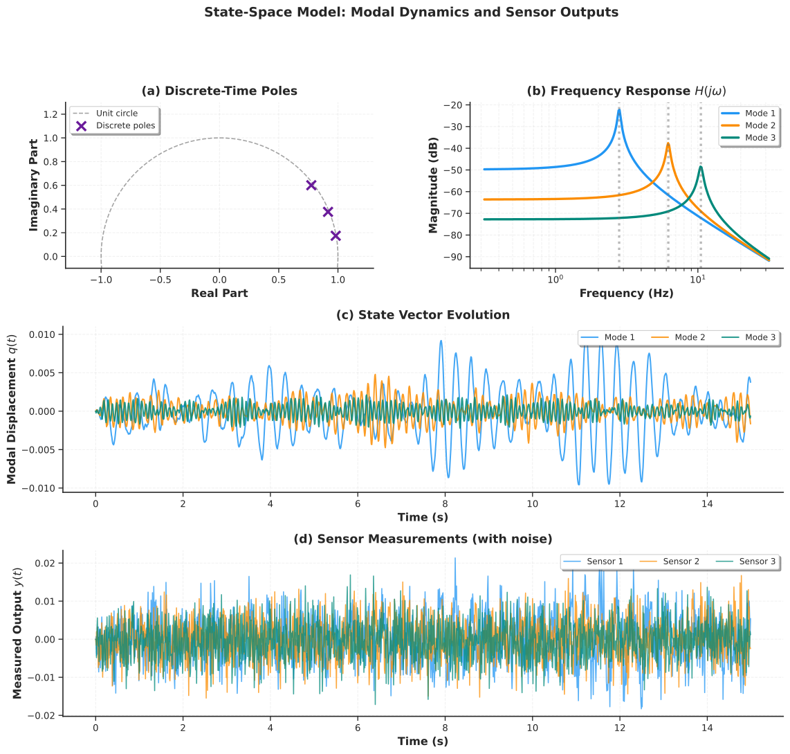
State-space model: modal dynamics and sensor outputs. (a) Discrete-time pole locations in the z-plane confirming stability. (b) Frequency response functions H(j\omega) for each mode showing resonance peaks at the natural frequencies. (c) State vector evolution showing modal displacement time histories. (d) Simulated sensor measurements including process and measurement noise. — Figure 9:State-space model: modal dynamics and sensor outputs. (a) Discrete-time pole locations in the $z$ -plane confirming stability. (b) Frequency response functions $H(j\omega)$ for each mode showing resonance peaks at the natural frequencies. (c) State vector evolution showing modal displacement time histories. (d) Simulated sensor measurements including process and measurement noise.

7Kalman Filter for Virtual Sensing¶

7.1Motivation: Estimating the Unmeasured¶

Consider a 100-meter cable-stayed bridge instrumented with only five accelerometers. Engineers need the vertical displacement at midspan, but that location has no sensor. Integrating the noisy acceleration measurements twice would accumulate drift, making displacement estimates worthless within seconds. The Kalman filter solves this problem by fusing sparse, noisy sensor data with a physics-based state-space model to produce optimal state estimates, including at locations where no physical sensor exists. This is virtual sensing: creating reliable measurements at uninstrumented locations.

The Kalman filter is optimal in the sense that it minimizes the mean-squared estimation error under the assumption that process and measurement noise are Gaussian. It operates recursively, processing one measurement at a time, which makes it suitable for real-time applications. And it provides uncertainty quantification for every state estimate, through the error covariance matrix, so that engineers know how much to trust each virtual measurement.

7.2Physical Intuition: Weighting Model Against Data¶

The Kalman filter can be understood as a weighted average between two sources of information at each time step. The physics-based model predicts where the state should be, and the sensors report where it actually appears to be. The relative trust placed in model versus sensors depends on their respective uncertainties, and this weighting is computed automatically through the Kalman gain matrix $\mathbf{K}_k$ .

When the model is accurate and the sensors are noisy, the Kalman gain is small and the filter trusts the model prediction. When the sensors are precise but the model has errors, the gain is large and the filter trusts the measurements. In steady state, the filter reaches an equilibrium where the reduction in uncertainty from each new measurement exactly balances the growth in uncertainty from each prediction step.

Kalman filter recursive algorithm: a two-stage predict-update cycle. The prediction step propagates state and covariance forward through the system model (\hat{\mathbf{x}}_{k|k-1} = \mathbf{A}\hat{\mathbf{x}}_{k-1} + \mathbf{B}\mathbf{u}_{k-1}, \mathbf{P}_{k|k-1} = \mathbf{A}\mathbf{P}_{k-1}\mathbf{A}^\top + \mathbf{Q}); the update step incorporates the new measurement \mathbf{y}_k via the Kalman gain \mathbf{K}_k, which optimally weights model predictions against sensor data. 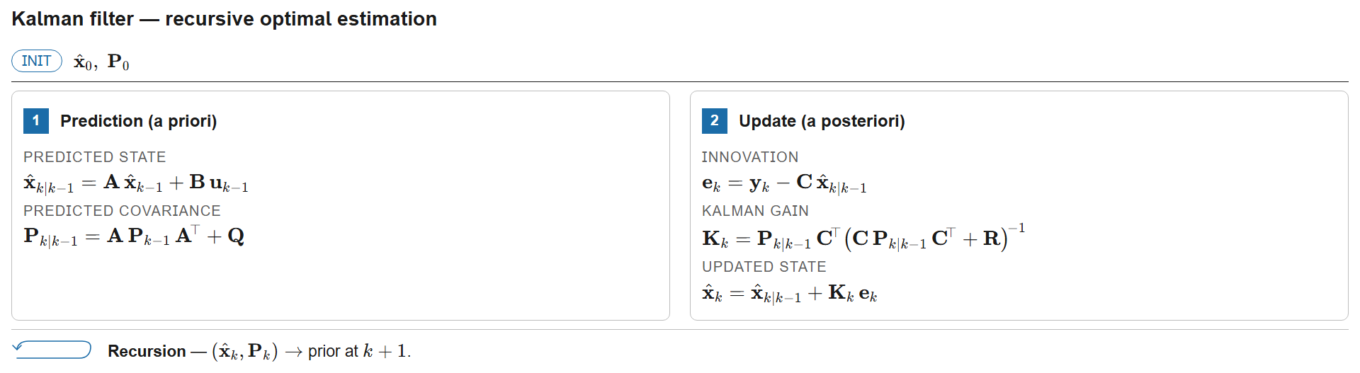— Figure 10:Kalman filter recursive algorithm: a two-stage predict-update cycle. The prediction step propagates state and covariance forward through the system model ( $\hat{\mathbf{x}}_{k|k-1} = \mathbf{A}\hat{\mathbf{x}}_{k-1} + \mathbf{B}\mathbf{u}_{k-1}$ , $\mathbf{P}_{k|k-1} = \mathbf{A}\mathbf{P}_{k-1}\mathbf{A}^\top + \mathbf{Q}$ ); the update step incorporates the new measurement $\mathbf{y}_k$ via the Kalman gain $\mathbf{K}_k$ , which optimally weights model predictions against sensor data.

7.3Mathematical Framework: Two-Stage Recursion¶

Given the discrete-time state-space model with noise:

\begin{aligned} \mathbf{z}_{k+1} &= \mathbf{A}_d \mathbf{z}_k + \mathbf{B}_d \mathbf{u}_k + \mathbf{w}_k, \quad \mathbf{w}_k \sim \mathcal{N}(\mathbf{0}, \mathbf{Q}) \\ \mathbf{y}_k &= \mathbf{H}_d \mathbf{z}_k + \mathbf{v}_k, \quad \mathbf{v}_k \sim \mathcal{N}(\mathbf{0}, \mathbf{R}) \end{aligned}

(20)

where $\mathbf{Q}$ is the process noise covariance (modeling unmodeled dynamics, disturbances, and model errors) and $\mathbf{R}$ is the measurement noise covariance (sensor inaccuracies, quantization, electromagnetic interference), the Kalman filter computes the state estimate $\hat{\mathbf{z}}_{k|k}$ that minimizes the mean-squared error.

Stage 1: Prediction (Time Update). The model propagates the state and covariance forward in time:

\begin{aligned} \hat{\mathbf{z}}_{k|k-1} &= \mathbf{A}_d \hat{\mathbf{z}}_{k-1|k-1} + \mathbf{B}_d \mathbf{u}_{k-1} \\ \mathbf{P}_{k|k-1} &= \mathbf{A}_d \mathbf{P}_{k-1|k-1} \mathbf{A}_d^\top + \mathbf{Q} \end{aligned}

(21)

The first equation applies the system dynamics to forecast the state. The second equation shows that prediction uncertainty grows due to process noise $\mathbf{Q}$ ; without new measurements, confidence in the state estimate deteriorates over time.

Stage 2: Update (Measurement Correction). A new measurement $\mathbf{y}_k$ is incorporated to refine the prediction:

\begin{aligned} \mathbf{K}_k &= \mathbf{P}_{k|k-1}\mathbf{H}_d^\top(\mathbf{H}_d\mathbf{P}_{k|k-1}\mathbf{H}_d^\top + \mathbf{R})^{-1} \\ \hat{\mathbf{z}}_{k|k} &= \hat{\mathbf{z}}_{k|k-1} + \mathbf{K}_k(\mathbf{y}_k - \mathbf{H}_d\hat{\mathbf{z}}_{k|k-1}) \\ \mathbf{P}_{k|k} &= (\mathbf{I} - \mathbf{K}_k\mathbf{H}_d)\mathbf{P}_{k|k-1} \end{aligned}

(22)

The Kalman gain $\mathbf{K}_k$ is the optimal weighting matrix. The quantity $\mathbf{y}_k - \mathbf{H}_d\hat{\mathbf{z}}_{k|k-1}$ is the innovation (measurement residual), representing the surprise in the new data. The updated estimate $\hat{\mathbf{z}}_{k|k}$ moves from the prediction toward the measurement by an amount proportional to the Kalman gain times the innovation. In the limiting case where $\mathbf{R} \to \infty$ (terrible sensors), the gain approaches zero and the filter ignores measurements entirely. When $\mathbf{Q} \to \infty$ (terrible model), the gain approaches $\mathbf{H}_d^{-1}$ and the filter ignores the model entirely.

For numerical stability in long simulations, the Joseph form of the covariance update is preferred:

\mathbf{P}_{k|k} = (\mathbf{I} - \mathbf{K}_k\mathbf{H}_d)\mathbf{P}_{k|k-1}(\mathbf{I} - \mathbf{K}_k\mathbf{H}_d)^\top + \mathbf{K}_k\mathbf{R}\mathbf{K}_k^\top

(23)

This formulation guarantees that $\mathbf{P}$ remains positive definite despite floating-point round-off errors. The computational cost per time step is dominated by the matrix inversion in the Kalman gain, which has dimension $n_y \times n_y$ where $n_y$ is the number of sensors. When the number of sensors is much smaller than the number of states ( $n_y \ll n_z$ ), the filter is efficient.

Algorithm 5 (Kalman Filter for Virtual Sensing)

Input: State-space model $(\mathbf{A}_d, \mathbf{B}_d, \mathbf{H}_d)$ , measurements $\{\mathbf{y}_k\}$ , inputs $\{\mathbf{u}_k\}$ , noise covariances $(\mathbf{Q}, \mathbf{R})$

Output: State estimates $\{\hat{\mathbf{z}}_{k|k}\}$ with uncertainties $\{\mathbf{P}_{k|k}\}$

Initialize:
- $\hat{\mathbf{z}}_{0|0} = \mathbb{E}[\mathbf{z}_0]$ (expected initial state)
- $\mathbf{P}_{0|0} = \text{Cov}[\mathbf{z}_0]$ (initial uncertainty)
For each timestep $k = 1, 2, \ldots, N$ :
a. Prediction (Time Update):
- State forecast: $\hat{\mathbf{z}}_{k|k-1} = \mathbf{A}_d \hat{\mathbf{z}}_{k-1|k-1} + \mathbf{B}_d \mathbf{u}_{k-1}$
- Covariance forecast: $\mathbf{P}_{k|k-1} = \mathbf{A}_d \mathbf{P}_{k-1|k-1} \mathbf{A}_d^\top + \mathbf{Q}$
b. Update (Measurement Correction):
- Innovation: $\mathbf{e}_k = \mathbf{y}_k - \mathbf{H}_d \hat{\mathbf{z}}_{k|k-1}$
- Innovation covariance: $\mathbf{S}_k = \mathbf{H}_d \mathbf{P}_{k|k-1} \mathbf{H}_d^\top + \mathbf{R}$
- Kalman gain: $\mathbf{K}_k = \mathbf{P}_{k|k-1} \mathbf{H}_d^\top \mathbf{S}_k^{-1}$
- State update: $\hat{\mathbf{z}}_{k|k} = \hat{\mathbf{z}}_{k|k-1} + \mathbf{K}_k \mathbf{e}_k$
- Covariance update (Joseph form): $\mathbf{P}_{k|k} = (\mathbf{I} - \mathbf{K}_k \mathbf{H}_d)\mathbf{P}_{k|k-1}(\mathbf{I} - \mathbf{K}_k \mathbf{H}_d)^\top + \mathbf{K}_k \mathbf{R} \mathbf{K}_k^\top$
Virtual sensing: For unmeasured DOFs with virtual measurement matrix $\mathbf{H}^{(v)}$ :
- Virtual measurement: $\hat{\mathbf{y}}_k^{(v)} = \mathbf{H}^{(v)} \hat{\mathbf{z}}_{k|k}$
- Uncertainty: $\boldsymbol{\Sigma}_k^{(v)} = \mathbf{H}^{(v)} \mathbf{P}_{k|k} (\mathbf{H}^{(v)})^\top$
Validation:
- Verify innovation whiteness: $\mathbb{E}[\mathbf{e}_k \mathbf{e}_j^\top] = \mathbf{0}$ for $j \neq k$
- Check normalized innovations: $\mathbf{e}_k^\top \mathbf{S}_k^{-1} \mathbf{e}_k \sim \chi^2_{n_y}$
- If validation fails, retune $\mathbf{Q}$ , $\mathbf{R}$ or refine model

kalman_filter.py

1
2
3
4
5
6
7
8
9
10
11
12
13
14
15
16
17
18
19
20
21
22
23
24
25
26
27
28
29
30
31
32
33
34
35
36
37
38
39
40
41
42
43
44
45
46
47
48
49
50
51
52
53
54
55
56
57
58
59
60
61
62
63
64
65
66
67
68
69
70
71
72
73
74
75
76
77
78
79
80
81
82
83
84
85
86
87
88
89
90
91
92
93
94
95
96
97
98
99
100
101
102
103
104
105
106
107
108
109
110
111
112
113
114
115
116
117
118
119
120
121
122
123
124
125
126
127
128
129
130
131
132
133
134
135
136
137
138
139
140
141
142
143
144
145
146
147
148
149
150
151
152
153
154
155
156
157
158
159
160
161
162
163
164
165
166
167
168
169
170
171
172
173
174
175
176
177
178
179
180
181
182
183
184
185
186
187
188
189
190
191
192
193
194
195
196
197
198
199
200
201
202
203
204
205
206
207
208
209
210
211
212
213
214
215
216
217
218
"""
Kalman Filter for Virtual Sensing - Chapter 8.

Provides the KalmanFilter class and a virtual sensing demonstration
that estimates unmeasured modal displacements from partial observations.
"""

import numpy as np
import matplotlib.pyplot as plt
from scipy import signal, linalg, stats
from statsmodels.tsa.stattools import acf
from typing import Tuple, Optional
import os

from utils import setup_plotting, COLORS, remove_spines, get_output_dir
from state_space_model import ModalStateSpaceModel


class KalmanFilter:
    """Discrete Kalman filter for linear state-space systems."""

    def __init__(self, A, B, H, Q, R, z0=None, P0=None):
        self.A, self.B, self.H = A, B, H
        self.Q, self.R = Q, R
        self.n_states = A.shape[0]
        self.n_outputs = H.shape[0]
        self.z_hat = z0 if z0 is not None else np.zeros(self.n_states)
        self.P = P0 if P0 is not None else np.eye(self.n_states)
        self.innovations = []
        self.innovation_covariances = []
        self.kalman_gains = []

    def predict(self, u=None):
        self.z_pred = self.A @ self.z_hat + (self.B @ u if u is not None else 0)
        self.P_pred = self.A @ self.P @ self.A.T + self.Q
        return self.z_pred, self.P_pred

    def update(self, y):
        innovation = y - self.H @ self.z_pred
        S = self.H @ self.P_pred @ self.H.T + self.R
        K = self.P_pred @ self.H.T @ linalg.inv(S)
        self.z_hat = self.z_pred + K @ innovation
        I_KH = np.eye(self.n_states) - K @ self.H
        self.P = I_KH @ self.P_pred @ I_KH.T + K @ self.R @ K.T
        self.innovations.append(innovation)
        self.innovation_covariances.append(S)
        self.kalman_gains.append(K)
        return self.z_hat, self.P

    def filter_sequence(self, measurements, inputs=None):
        n_steps = measurements.shape[0]
        state_estimates = np.zeros((n_steps, self.n_states))
        covariances = np.zeros((n_steps, self.n_states, self.n_states))
        self.innovations, self.innovation_covariances, self.kalman_gains = [], [], []
        for k in range(n_steps):
            u_k = inputs[k] if inputs is not None else None
            self.predict(u_k)
            self.update(measurements[k])
            state_estimates[k] = self.z_hat
            covariances[k] = self.P
        return state_estimates, covariances

    def get_virtual_sensor(self, state_estimates, covariances, H_virtual):
        n_steps = state_estimates.shape[0]
        n_virtual = H_virtual.shape[0]
        outputs = np.zeros((n_steps, n_virtual))
        uncertainties = np.zeros((n_steps, n_virtual, n_virtual))
        for k in range(n_steps):
            outputs[k] = H_virtual @ state_estimates[k]
            uncertainties[k] = H_virtual @ covariances[k] @ H_virtual.T
        return outputs, uncertainties


def virtual_sensing_demo():
    """
    Demonstrate virtual sensing with partial measurements.
    3-mode bridge, only modes 1 and 3 measured, mode 2 estimated.
    """
    model = ModalStateSpaceModel(
        frequencies_hz=np.array([3.2, 7.1, 11.8]),
        damping_ratios=np.array([0.02, 0.028, 0.035])
    ).discretize(dt=0.01)

    rng = np.random.default_rng(500)
    n_steps = 5000
    true_input = signal.lfilter([1], [1, -0.8], rng.standard_normal((n_steps, 3)))
    true_states, true_outputs = model.simulate(
        true_input, process_noise_std=1e-5, measurement_noise_std=3e-3, seed=500)

    measured_idx = [0, 2]
    H_partial = model.H_d[measured_idx, :]
    measurements = true_outputs[:, measured_idx]

    Q = 1e-8 * np.eye(model.A_d.shape[0])
    R = (3e-3)**2 * np.eye(len(measured_idx))

    kf = KalmanFilter(A=model.A_d, B=model.B_d, H=H_partial, Q=Q, R=R,
                      z0=np.zeros(model.A_d.shape[0]),
                      P0=np.eye(model.A_d.shape[0]) * 0.1)

    est_states, est_cov = kf.filter_sequence(measurements, true_input)

    virtual = est_states[:, 2]
    true_unmeasured = true_states[:, 2]
    virtual_std = np.sqrt(est_cov[:, 2, 2])
    error = true_unmeasured - virtual

    return {
        'true_unmeasured': true_unmeasured, 'virtual_output': virtual,
        'virtual_std': virtual_std, 'estimation_error': error,
        'measurements': measurements, 'innovations': np.array(kf.innovations),
        'rmse': np.sqrt(np.mean(error**2)),
        'correlation': np.corrcoef(true_unmeasured, virtual)[0, 1],
        'dt': model.dt
    }


def generate_kalman_figure():
    """Generate the Kalman filter virtual sensing figure."""
    setup_plotting()
    res = virtual_sensing_demo()

    print(f"RMSE: {res['rmse']:.6f}, Correlation: {res['correlation']:.4f}")

    fig = plt.figure(figsize=(14, 14))
    gs = fig.add_gridspec(4, 2, hspace=0.4, wspace=0.3)
    dt = res['dt']
    t = np.arange(len(res['true_unmeasured'])) * dt

    # (a) Physical sensors
    ax1 = fig.add_subplot(gs[0, :])
    ax1.plot(t[:1200], res['measurements'][:1200, 0], linewidth=1.5,
             label='Sensor 1 (Mode 1)', color=COLORS['primary'], alpha=0.85)
    ax1.plot(t[:1200], res['measurements'][:1200, 1], linewidth=1.5,
             label='Sensor 2 (Mode 3)', color=COLORS['accent'], alpha=0.85)
    ax1.set_ylabel('Measurement')
    ax1.set_title('(a) Physical Sensor Measurements', pad=8)
    ax1.legend(loc='upper right', frameon=True, shadow=True, fontsize=10, fancybox=True, ncol=2)
    ax1.grid(True, alpha=0.3, linestyle='--')
    remove_spines(ax1)

    # (b) True vs virtual with confidence band
    ax2 = fig.add_subplot(gs[1, :])
    ax2.plot(t[:1200], res['true_unmeasured'][:1200], linewidth=2.5,
             label='True (Mode 2)', color=COLORS['true'], alpha=0.9)
    ax2.plot(t[:1200], res['virtual_output'][:1200], linewidth=2.0,
             label='Virtual Sensor', color=COLORS['estimated'], linestyle='--', alpha=0.85)
    ax2.set_ylabel('Displacement')
    ax2.set_title('(b) Virtual Sensor Reconstruction (Unmeasured Mode 2)', pad=8)
    ax2.legend(loc='upper right', frameon=True, shadow=True, fontsize=10, fancybox=True)
    ax2.grid(True, alpha=0.3, linestyle='--')
    remove_spines(ax2)

    # (c) Error
    ax3 = fig.add_subplot(gs[2, 0])
    std_err = np.std(res['estimation_error'])
    ax3.plot(t, res['estimation_error'], linewidth=0.8, color=COLORS['warning'], alpha=0.7)
    ax3.axhline(0, color='k', linestyle='--', linewidth=1.0)
    ax3.fill_between(t, -2 * std_err, 2 * std_err, alpha=0.15, color=COLORS['warning'])
    ax3.set_xlabel('Time (s)')
    ax3.set_ylabel('Error')
    ax3.set_title('(c) Estimation Error', pad=8)
    ax3.grid(True, alpha=0.3, linestyle='--')
    remove_spines(ax3)

    # (d) Error histogram
    ax4 = fig.add_subplot(gs[2, 1])
    ax4.hist(res['estimation_error'], bins=50, density=True,
             color=COLORS['neutral'], alpha=0.7, edgecolor='black', linewidth=0.5)
    x_norm = np.linspace(res['estimation_error'].min(), res['estimation_error'].max(), 200)
    ax4.plot(x_norm, stats.norm.pdf(x_norm, 0, std_err), color=COLORS['warning'],
             linewidth=2.5, label='Gaussian fit')
    ax4.set_xlabel('Error')
    ax4.set_ylabel('Density')
    ax4.set_title('(d) Error Distribution', pad=8)
    ax4.legend(loc='upper right', frameon=True, shadow=True, fontsize=10, fancybox=True)
    ax4.grid(True, alpha=0.3, linestyle='--', axis='y')
    remove_spines(ax4)

    # (e) Innovation sequence
    ax5 = fig.add_subplot(gs[3, 0])
    innov = res['innovations'][:, 0]
    ax5.plot(t[:2000], innov[:2000], linewidth=0.7, color=COLORS['secondary'], alpha=0.65)
    ax5.axhline(0, color='k', linestyle='--', linewidth=1.0)
    ax5.set_xlabel('Time (s)')
    ax5.set_ylabel('Innovation')
    ax5.set_title('(e) Innovation Sequence (Sensor 1)', pad=8)
    ax5.grid(True, alpha=0.3, linestyle='--')
    remove_spines(ax5)

    # (f) Innovation ACF
    ax6 = fig.add_subplot(gs[3, 1])
    inn_acf = acf(innov, nlags=40, fft=True)
    lags = np.arange(len(inn_acf))
    ml, sl, bl = ax6.stem(lags, inn_acf, linefmt='-', markerfmt='o', basefmt=' ')
    sl.set_color(COLORS['secondary']); sl.set_linewidth(1.5)
    ml.set_color(COLORS['secondary']); ml.set_markersize(3)
    ci = 1.96 / np.sqrt(len(innov))
    ax6.axhline(ci, color=COLORS['warning'], linestyle='--', linewidth=1.5, alpha=0.7)
    ax6.axhline(-ci, color=COLORS['warning'], linestyle='--', linewidth=1.5, alpha=0.7)
    ax6.set_xlabel('Lag')
    ax6.set_ylabel('ACF')
    ax6.set_title('(f) Innovation Whiteness Check', pad=8)
    ax6.grid(True, alpha=0.3, linestyle='--')
    remove_spines(ax6)

    fig.suptitle('Kalman Filter Virtual Sensing: Performance Evaluation',
                 fontsize=14, fontweight='bold', y=1.00)

    output_path = os.path.join(get_output_dir(), 'ch08_fig_virtual_sensing.svg')
    plt.savefig(output_path, bbox_inches='tight')
    plt.close()
    print(f"Saved: {output_path}")
    return output_path


if __name__ == '__main__':
    generate_kalman_figure()

Kalman filter virtual sensing: performance evaluation. (a) Physical sensor measurements from instrumented modes 1 and 3. (b) Virtual sensor reconstruction of the unmeasured mode 2 displacement with 95% confidence interval. (c) Estimation error with \pm 2\sigma bounds. (d) Error distribution with Gaussian fit. (e) Innovation sequence for sensor 1. (f) Innovation autocorrelation function verifying whiteness of the filter residuals. 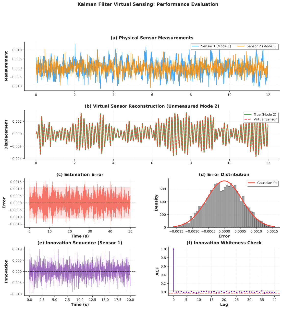— Figure 11:Kalman filter virtual sensing: performance evaluation. (a) Physical sensor measurements from instrumented modes 1 and 3. (b) Virtual sensor reconstruction of the unmeasured mode 2 displacement with 95% confidence interval. (c) Estimation error with $\pm 2\sigma$ bounds. (d) Error distribution with Gaussian fit. (e) Innovation sequence for sensor 1. (f) Innovation autocorrelation function verifying whiteness of the filter residuals.

8Practical Considerations and Best Practices¶

8.1Choosing the Right Model¶

The five model families developed in this chapter form a hierarchy of increasing capability and complexity. Selecting the right level depends on the monitoring objective, the available measurements, and the computational budget.

AR models are the simplest choice and should be the starting point for any parametric analysis. They require only a single output channel, can be estimated by solving a linear system, and produce modal parameters directly through the pole mapping. AR models are sufficient when the excitation is approximately white, the structure is linear and stationary, and the goal is modal identification or simple anomaly detection via residual monitoring.

ARMA models extend AR by explicitly modeling colored excitation. They should be considered when the Ljung-Box test on AR residuals fails, indicating that temporal correlation remains unexplained. The improvement comes at the cost of nonlinear estimation (iterative MLE rather than linear regression) and an additional model order to select. In practice, ARMA is most useful when the excitation spectrum has strong peaks or valleys that the AR model cannot capture without an unreasonably high order.

ARMAX models incorporate measured exogenous inputs and are the preferred choice for damage detection when operational variability is large and input measurements (traffic loads, wind speed, temperature) are available. By accounting for known sources of response variation, ARMAX residuals become sensitive primarily to structural changes, which reduces false alarm rates. The additional cost is a three-dimensional order search $(p, q, r)$ and the requirement for synchronized input-output data.

State-space models, combined with Kalman filtering, are necessary when the application requires multi-sensor fusion, virtual sensing at uninstrumented locations, or real-time state estimation with uncertainty quantification. They require a physics-based model (mass, stiffness, and damping matrices or modal parameters), which is typically obtained from finite element analysis (Chapter 6) or from operational modal analysis. The Kalman filter adds the ability to process measurements recursively and to estimate quantities that are not directly measured.

8.2Noise Covariance Tuning for Kalman Filters¶

The performance of the Kalman filter depends critically on the process noise covariance $\mathbf{Q}$ and the measurement noise covariance $\mathbf{R}$ . The ratio $\mathbf{Q}/\mathbf{R}$ controls the balance between model trust and measurement trust.

For the measurement noise covariance $\mathbf{R}$ , sensor specification sheets usually provide noise floor or resolution values that can be used directly. If sensors are uncorrelated, $\mathbf{R}$ is diagonal with entries equal to the squared noise standard deviation of each sensor. A more empirical approach is to record data under zero-input conditions (the structure at rest) and estimate the sensor noise covariance from these recordings.

For the process noise covariance $\mathbf{Q}$ , there is no direct physical measurement. A common starting point is $\mathbf{Q} = \alpha \mathbf{I}$ with $\alpha$ between 10^-6 and 10^-4. Increasing $\alpha$ makes the filter more responsive to rapid changes (useful for time-varying systems) but also more sensitive to measurement noise. Decreasing $\alpha$ makes the filter smoother but slower to track genuine changes. A principled approach is innovation-based tuning: if the filter is well-tuned, the innovation sequence $\{\mathbf{e}_k\}$ should be white with covariance $\mathbf{S}_k$ . If the innovations show significant autocorrelation, $\mathbf{Q}$ is too small; if the innovations are excessively noisy relative to $\mathbf{S}_k$ , $\mathbf{Q}$ is too large.

8.3Computational Efficiency for Real-Time SHM¶

For real-time deployment on embedded hardware or edge computing devices, several strategies reduce computational cost. Steady-state Kalman gain pre-computation is the most effective: for time-invariant systems, the Kalman gain converges to a constant matrix $\mathbf{K}_\infty$ after a transient period (typically a few hundred steps). Once converged, the gain matrix can be pre-computed offline and stored, eliminating the matrix inversion at each time step and reducing the online cost to two matrix-vector multiplications per step. Reduced-order modeling via modal truncation retains only the $m$ dominant modes (those with frequencies below a cutoff, for example $f_n < 20$ Hz), which reduces the state dimension from $2n$ (where $n$ may be thousands for a full FE model) to $2m$ (where $m$ is typically 5 to 20). Square-root filtering reformulates the covariance update in terms of the Cholesky factor of $\mathbf{P}$ , which improves numerical stability and can be more efficient for certain matrix dimensions. Finally, exploiting the block-diagonal structure of modal state-space models allows each mode to be filtered independently, enabling parallel computation.

8.4Common Pitfalls¶

Non-stationarity is perhaps the most frequent source of error. Temperature variations, changing traffic patterns, and seasonal effects cause the structural properties to drift slowly over time. If the monitoring window is too long, AR coefficients estimated from the first half of the data may not describe the second half accurately. Short, overlapping analysis windows with periodic model re-estimation help mitigate this issue.

Sensor failure and data loss require special handling in the Kalman filter framework. When a sensor drops out temporarily, the corresponding row of the measurement matrix $\mathbf{H}_d$ should be removed for those time steps, and the filter will rely more heavily on the model prediction. The uncertainty in the affected states will grow during the outage and recover when the sensor returns.

Numerical conditioning can become an issue for high-dimensional state-space models. The covariance matrix $\mathbf{P}$ can lose positive definiteness due to accumulated round-off errors, causing the filter to diverge. The Joseph form of the covariance update (used in the implementation above) helps, but for very long simulations or ill-conditioned systems, square-root filtering may be necessary.

8.5Software and Implementation Notes¶

Several Python libraries provide reliable, well-tested implementations of the methods discussed in this chapter. The statsmodels library offers AutoReg for AR models, ARIMA for ARMA models, and SARIMAX for ARMAX models, all with built-in order selection, diagnostic tests, and maximum likelihood estimation. For Kalman filtering, filterpy provides a well-tested implementation with support for extended and unscented variants, while scipy.signal includes functions for state-space model construction (cont2discrete, dlsim) and spectral analysis (welch, periodogram). The custom KalmanFilter and ModalStateSpaceModel classes developed in this chapter are intended as pedagogical tools; for production SHM systems, the tested library implementations should be preferred.

9Summary¶

9.1Chapter Synthesis¶

This chapter developed five progressively richer parametric model families for structural health monitoring, each building on the one before. AR models provided the entry point: a linear, output-only representation whose coefficients map to natural frequencies and damping ratios through the logarithmic pole transformation. ARMA models extended AR by adding moving-average terms to capture colored excitation, improving residual whiteness at the cost of nonlinear estimation. ARMAX models incorporated measured exogenous inputs, enabling damage detection that is robust to operational variability because the known loading is explicitly modeled. State-space representations reformulated the problem in matrix form, connecting data-driven models to the physics of structural dynamics and enabling multi-sensor, multi-output analysis. The Kalman filter, operating on the state-space model, provided optimal recursive state estimation with uncertainty quantification, making virtual sensing and real-time monitoring practical.

The unifying theme across all five models is the exploitation of temporal structure in vibration data. A lightly damped structure has memory: its current state depends predictably on its recent past. Parametric models encode this memory in a compact set of coefficients, and from those coefficients we extract the physical properties of the structure. When those properties change, we detect damage. When combined with a physics-based model, we can estimate quantities that are never directly measured.

9.2From Sensors to Decisions: The Complete SHM Pipeline¶

Looking back across the entire book, the tools developed in each chapter correspond to a stage in the SHM decision pipeline. Chapters 1 and 2 established the sensing foundation: what physical quantities to measure, how transducers convert them to electrical signals, and how to condition and digitize those signals reliably. Chapter 3 introduced time-domain analysis for preprocessing, trend removal, and basic statistical characterization. Chapter 4 developed frequency-domain methods for modal identification and spectral analysis, providing the non-parametric perspective that this chapter’s parametric methods complement and extend. Chapter 5 focused on feature engineering and anomaly detection, extracting damage-sensitive features from raw data and establishing statistical baselines. Chapter 6 addressed finite element model updating and optimal sensor placement, connecting computational models to experimental measurements and ensuring that sensor networks provide maximum information. Chapter 7 introduced machine learning classification for pattern recognition and data-driven decision making.

This final chapter completes the pipeline by providing the mathematical framework for fusing all of these elements. The parametric models encode structural physics in compact, interpretable form. The Kalman filter combines physics-based predictions with real-time sensor data to produce optimal state estimates. Together, they enable the transition from passive monitoring (collecting data and looking for anomalies) to active estimation (computing the current state of the structure and quantifying confidence in that estimate).

9.3Research Frontiers¶

The linear Gaussian framework developed in this chapter represents the established foundation, but several active research directions extend these ideas to more complex scenarios. The Extended Kalman Filter (EKF) and Unscented Kalman Filter (UKF) handle nonlinear dynamics by linearizing the state-space model locally or by propagating carefully chosen sigma points through the nonlinear function. Particle filters (sequential Monte Carlo methods) can handle arbitrary distributions and strong nonlinearity, at higher computational cost. Bayesian model updating combines parametric models with probabilistic inference to update model parameters as new data arrives, quantifying epistemic uncertainty in the model itself rather than just the state. Digital twins integrate real-time sensor data with high-fidelity finite element models, creating a continuously updated virtual replica of the physical structure that can be used for prognosis and remaining-life estimation. Physics-informed neural networks blend deep learning with governing equations, offering a hybrid approach that can learn complex input-output relationships while respecting conservation laws and boundary conditions. Population-based SHM extends monitoring from individual structures to fleets, using data from similar structures to improve damage detection on structures with limited instrumentation.

9.4Closing Thoughts¶

The infrastructure that modern society depends on, including bridges, buildings, wind turbines, pipelines, and power plants, is aging. The engineering challenge of the coming decades is to maintain and extend the service life of these structures safely and economically. Structural health monitoring, powered by the sensing and data analytics tools developed throughout this book, provides the technical foundation for meeting that challenge. The parametric models and optimal filters presented in this chapter represent the current state of the art for real-time, physics-informed monitoring. As sensor technology becomes cheaper, computation more powerful, and algorithms more sophisticated, the vision of continuously monitored, self-diagnosing infrastructure moves steadily closer to reality.

10Exercises¶

11References¶

Ljung, L. (1999). System Identification: Theory for the User (2nd ed.). Prentice Hall.
Kalman, R. E. (1960). A New Approach to Linear Filtering and Prediction Problems. Journal of Basic Engineering, 82(1), 35-45.
Peeters, B., & De Roeck, G. (2001). Stochastic System Identification for Operational Modal Analysis: A Review. Journal of Dynamic Systems, Measurement, and Control, 123(4), 659-667.
Van Overschee, P., & De Moor, B. (1996). Subspace Identification for Linear Systems. Springer.
Carden, E. P., & Brownjohn, J. M. W. (2008). ARMA Modelled Time-Series Classification for Structural Health Monitoring. Mechanical Systems and Signal Processing, 22(2), 295-314.
Chatzi, E. N., & Smyth, A. W. (2009). The Unscented Kalman Filter and Particle Filter Methods for Nonlinear Structural System Identification. Structural Control and Health Monitoring, 16(1), 99-123.
Azam, S. E., Chatzi, E., & Papadimitriou, C. (2015). A Dual Kalman Filter Approach for State Estimation via Output-Only Acceleration Measurements. Mechanical Systems and Signal Processing, 60-61, 866-886.
Reynders, E., Houbrechts, J., & De Roeck, G. (2012). Fully Automated (Operational) Modal Analysis. Mechanical Systems and Signal Processing, 29, 228-250.
Naets, F., Cuadrado, J., & Desmet, W. (2015). Stable Force Identification in Structural Dynamics Using Kalman Filtering and Dummy Measurements. Mechanical Systems and Signal Processing, 50-51, 235-248.
Brownjohn, J. M. W., De Stefano, A., Xu, Y. L., Wenzel, H., & Aktan, A. E. (2011). Vibration-Based Monitoring of Civil Infrastructure: Challenges and Successes. Journal of Civil Structural Health Monitoring, 1(3-4), 79-95.
Box, G. E. P., Jenkins, G. M., Reinsel, G. C., & Ljung, G. M. (2015). Time Series Analysis: Forecasting and Control (5th ed.). Wiley.
Simon, D. (2006). Optimal State Estimation: Kalman, H-Infinity, and Nonlinear Approaches. Wiley.
Sohn, H., Farrar, C. R., Hemez, F. M., Shunk, D. D., Stinemates, D. W., Nadler, B. R., & Czarnecki, J. J. (2004). A Review of Structural Health Monitoring Literature: 1996-2001. Los Alamos National Laboratory Report, LA-13976-MS.
Friswell, M. I., & Mottershead, J. E. (1995). Finite Element Model Updating in Structural Dynamics. Springer.
Worden, K., & Dulieu-Barton, J. M. (2004). An Overview of Intelligent Fault Detection in Systems and Structures. Structural Health Monitoring, 3(1), 85-98.
Mariani, S., & Ghisi, A. (2007). Unscented Kalman Filtering for Nonlinear Structural Dynamics. Nonlinear Dynamics, 49(1-2), 131-150.